Perform environmental filtering on species occurrences

This function perform filtering on species occurrences based on their environmental conditions.

Usage

occfilt_env(data, x, y, id, env_layer, nbins)

Arguments

data: data.frame. Data.frame or tibble object with presences (or presence-absence) records, and coordinates
x: character. Column name with spatial x coordinates
y: character. Column name with spatial y coordinates
id: character. Column names with rows id. It is important that each row has its own unique code.
env_layer: SpatRaster. Raster variables that will be used to fit the model. Factor variables will be removed.
nbins: integer. A number of classes used to split each environmental condition. It is possible to use single or several values. If several values are provided, the function will return a list with the results. Usage nbins = 5 or nbins = c(5, 10, 15)

Value

If one value is used to filter occurrence funtion will return a tibble object with filtered data. If several values are used to filter occurrences, the function will return a list of tibbles with filtered data.

Details

This function uses an approach adapted from the approach proposed by Varela et al. (2014). It consists of filtering occurrences in environmental space. First, a regular multidimensional grid is created in environmental space. This multidimensional grid is determined by the environmental variables (always use continuous variables) the grid cell size is defined by the number of bins, used for dividing variable range into interval classes (Varela et al. 2014; Castellanos et al., 2019). The number of bins is set in the "nbins" argument. Then, a single occurrence is randomly selected within each cell of the multidimensional grid. Consider that there is a trade-off between the number of bins and the number of filtered records because as the number of bins decreases, the cell size of the grids increases, and the number of filtered records decreases (Castellanos et al., 2019). occfilt_env works for any number of dimensions (variables) and with the original variables without performing a PCA beforehand.

The greater the number of predictor variables (i.e., the number of dimensions of the multidimensional environmental grid) and the greater the number of bins, the greater the time processing and the computer memory used. Therefore, it is recommended to use a small number of bins between 2-5 if more than ten variables are used.

Environmental filters are sensitive to the number of bins. A procedure for selecting the number of bins was used by Velazco et al. (2020) and it is implemented in occfilt_geo.

References

Castellanos, A. A., Huntley, J. W., Voelker, G., & Lawing, A. M. (2019). Environmental filtering improves ecological niche models across multiple scales. Methods in Ecology and Evolution, 10(4), 481-492. https://doi.org/10.1111/2041-210X.13142
Varela, S., Anderson, R. P., Garcia-Valdes, R., & Fernandez-Gonzalez, F. (2014). Environmental filters reduce the effects of sampling bias and improve predictions of ecological niche models. Ecography, 37, 1084-1091. https://doi.org/10.1111/j.1600-0587.2013.00441.x
Velazco, S. J. E., Svenning, J-C., Ribeiro, B. R., & Laureto, L. M. O. (2020). On opportunities and threats to conserve the phylogenetic diversity of Neotropical palms. Diversity and Distributions, 27, 512–523. https://doi.org/10.1111/ddi.13215

Examples

if (FALSE) { # \dontrun{
require(terra)
require(dplyr)
require(ggplot2)

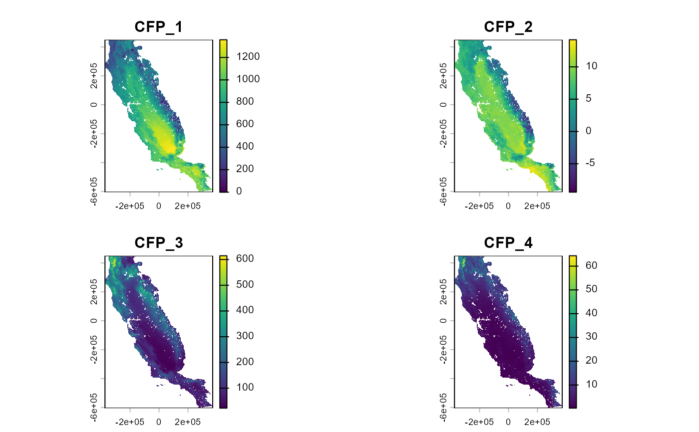
# Environmental variables
somevar <- system.file("external/somevar.tif", package = "flexsdm")
somevar <- terra::rast(somevar)

plot(somevar)

# Species occurrences
data("spp")
spp
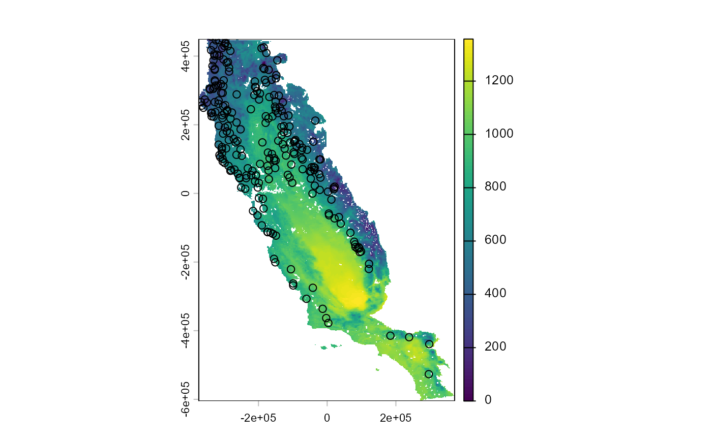
spp1 <- spp %>% dplyr::filter(species == "sp1", pr_ab == 1)

somevar[[1]] %>% plot()
points(spp1 %>% select(x, y))

spp1$idd <- 1:nrow(spp1)


# split environmental variables into 5 bins
filtered_1 <- occfilt_env(
  data = spp1,
  x = "x",
  y = "y",
  id = "idd",
  env_layer = somevar,
  nbins = 5
)

# split into 8 bins
filtered_2 <- occfilt_env(
  data = spp1,
  x = "x",
  y = "y",
  id = "idd",
  env_layer = somevar,
  nbins = 8
)

# split into 12 bins
filtered_3 <- occfilt_env(
  data = spp1,
  x = "x",
  y = "y",
  id = "idd",
  env_layer = somevar,
  nbins = 12
)


## %######################################################%##
####         ' # Test different number of bins          ####
## %######################################################%##

filtered_dif_bins <- occfilt_env(
  data = spp1,
  x = "x",
  y = "y",
  id = "idd",
  env_layer = somevar,
  nbins = c(4, 6, 8, 10, 12, 14)
)

class(filtered_dif_bins)
names(filtered_dif_bins) # each elements of this list has the names of the bins

filtered_dif_bins %>%
  dplyr::bind_rows(.id = "bins") %>%
  dplyr::mutate(bins = as.numeric(bins)) %>%
  ggplot(aes(x = x, y = y)) +
  geom_point() +
  facet_wrap(~bins)
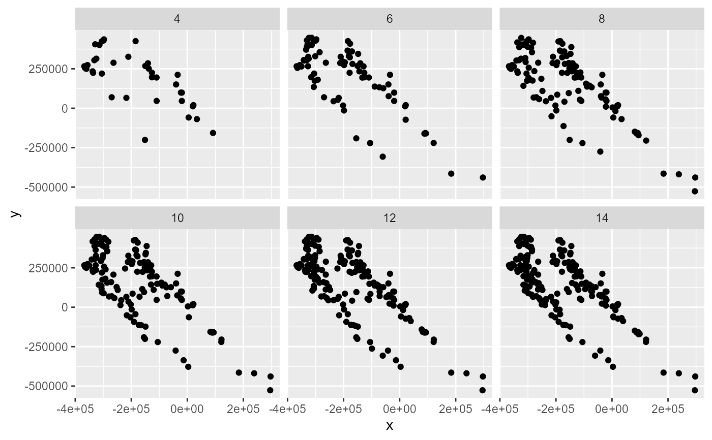# note that the higher the nbins parameter the more
# classes must be processed (4 variables, 30 bins = 923521 classes)

# While the greater the greater the number of bins, the greater records retained


# It is possible select the best of filtered
# datasets using the occfilt_selec function

occ_selected <- occfilt_select(
  occ_list = filtered_dif_bins,
  x = "x",
  y = "y",
  env_layer = somevar,
  filter_prop = TRUE
)

occ_selected
} # }