flexsdm: Modeling a rare species
Source:vignettes/v05_Rare_species_example.Rmd
v05_Rare_species_example.RmdIntro
Creating SDMs for rare or poorly known species can be a difficult task. Occurrence data are often limited to only a few observation, which can lead to model overfitting, especially when using many predictor variables to build models. However, researchers are often most interested in building SDMs for rare species, as they are often the most threatened and in need of conservation action.
To address the issues associated with modeling the spatial distributions of rare species, Lomba et al. (2010) and Breiner et al. (2015) proposed the method “ensemble of small models” or ESM. In ESM, many bivariate models with pairwise combinations of each predictor variable, then an ensemble is performed. In flexsdm, the ensemble is created using the average of suitability across all of the “small models”, weighted by Somers’ D (D = 2 * (AUC-.5)). It is important to note that this method does not allow the use of categorical variables (such as soil type).
The practical applications of ESMs could include identifying areas for reintroduction of rare species or areas for establishing new populations, especially in the face of climate change. For example, Dubos et al. (2021) used a variation of ESM to identify areas that may remain suitable under climate change for two rare species from Madagascar: the golden mantella frog (Mantella aurantiaca) and the Manapany day gecko (Phelsuma inexpectata).
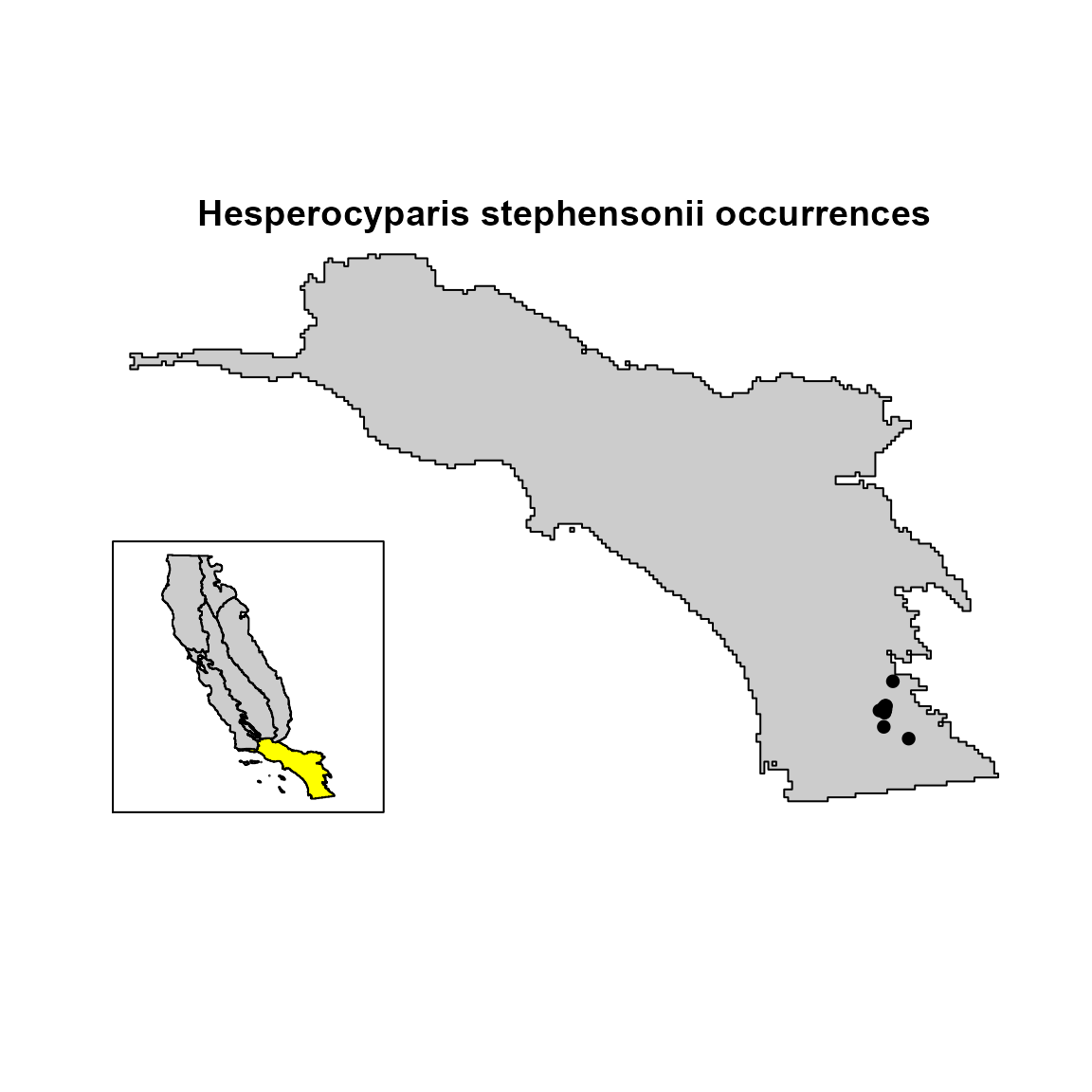
In this example, we will walk through the process of comparing ESM to traditional modeling approaches for Hesperocyparis stephensonii (Cuyamaca cypress), a conifer tree species that is endemic to southern California. This species is listed as Critically Endangered by the IUCN and is only found in the headwaters of King Creek in San Diego County. The Cedar Fire of 2003 left only 30-40 surviving trees. In this hypothetical example, we are searching for suitable areas where it might be possible to establish new populations of this species, with the hopes of decreasing the species’ future extinction risk.
Data
For our models, we will use four environmental variables that influence plant distributions in California: available evapotranspiration (aet), climatic water deficit (cwd), maximum temperature of the warmest month (tmx), and minimum temperature of the coldest month (tmn). Our occurrence data include 21 geo-referenced observations downloaded from the online database Calflora.
# devtools::install_github('sjevelazco/flexsdm')
library(flexsdm)
library(terra)
library(dplyr)

# environmental data
somevar <- system.file("external/somevar.tif", package = "flexsdm")
somevar <- terra::rast(somevar)
names(somevar) <- c("aet", "cwd", "tmx", "tmn")

# species occurence data (presence-only)
data(hespero)
hespero <- hespero %>% dplyr::select(-id)

# California ecoregions
regions <- system.file("external/regions.tif", package = "flexsdm")
regions <- terra::rast(regions)
regions <- as.polygons(regions)
sp_region <- terra::subset(regions, regions$category == "SCR") # ecoregion where *Hesperocyparis stephensonii* is found

# visualize the species occurrences
plot(
  sp_region,
  col = "gray80",
  legend = FALSE,
  axes = FALSE,
  main = "Hesperocyparis stephensonii occurrences"
)
points(hespero[, c("x", "y")], col = "black", pch = 16)
cols <- rep("gray80", 8)
cols[regions$category == "SCR"] <- "yellow"
terra::inset(
  regions,
  loc = "bottomleft",
  scale = .3,
  col = cols
)
Delimit calibration area
First, we must define our model’s calibration area. The flexsdm package offers several methods for defining the model calibration area. Here, we will use 25-km buffer areas around the presence points to select our pseudo-absence locations.
ca <- calib_area(
  data = hespero,
  x = "x",
  y = "y",
  method = c("buffer", width = 25000),
  crs = crs(somevar)
)

# visualize the species occurrences & calibration area
plot(
  sp_region,
  col = "gray80",
  legend = FALSE,
  axes = FALSE,
  main = "Calibration area and occurrences"
)
plot(ca, add = TRUE)
points(hespero[, c("x", "y")], col = "black", pch = 16)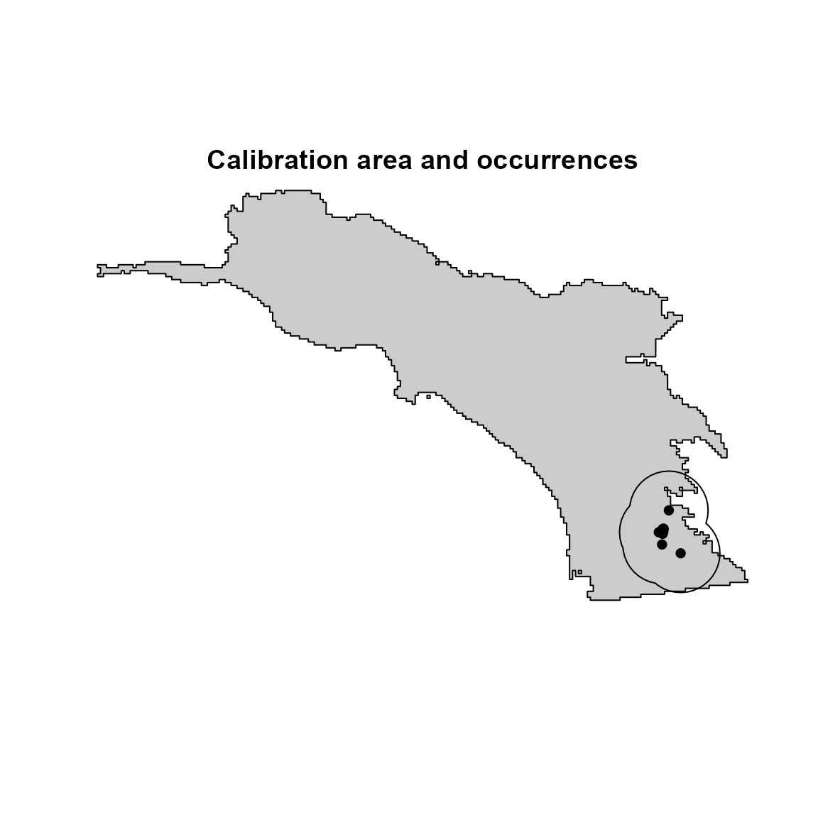
Create pseudo-absence data
As is often the case with rare species, we only have species presence data. However, most SDM methods require either pseudo-absence or background data. Here, we use our calibration area to produce pseudo-absence data that can be used in our SDMs.
# Sample the same number of species presences
set.seed(10)
psa <- sample_pseudoabs(
  data = hespero,
  x = "x",
  y = "y",
  n = sum(hespero$pr_ab), # selecting number of pseudo-absence points that is equal to number of presences
  method = "random",
  rlayer = somevar,
  calibarea = ca
)

# Visualize species presences and pseudo-absences
plot(
  sp_region,
  col = "gray80",
  legend = FALSE,
  axes = FALSE,
  xlim = c(289347, 353284),
  ylim = c(-598052, -520709),
  main = "Presence = yellow, Pseudo-absence = black"
)
plot(ca, add = TRUE)
points(psa[, c("x", "y")], cex = 0.8, pch = 16, col = "black") # Pseudo-absences
points(hespero[, c("x", "y")], col = "yellow", pch = 16, cex = 1.5) # Presences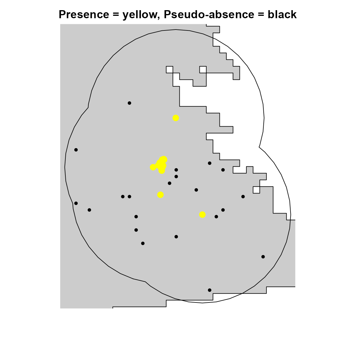
# Bind a presences and pseudo-absences
hespero_pa <- bind_rows(hespero, psa)
hespero_pa # Presence-Pseudo-absence database
#> # A tibble: 42 × 3
#>          x        y pr_ab
#>      <dbl>    <dbl> <dbl>
#>  1 316923. -557843.     1
#>  2 317155. -559234.     1
#>  3 316960. -558186.     1
#>  4 314347. -559648.     1
#>  5 317348. -557349.     1
#>  6 316753. -559679.     1
#>  7 316777. -558644.     1
#>  8 317050. -559043.     1
#>  9 316655. -559928.     1
#> 10 316418. -567439.     1
#> # ℹ 32 more rows
Partition data for evaluating models
To evaluate model performance, we need to specify data for testing and training. flexsdm offers a range of random and spatial and random data partition methods for evaluating SDMs. Here we will use repeated K-fold cross-validation, which is a suitable partition approach for performing ESM.
set.seed(10)

# Repeated K-fold method
hespero_pa2 <- part_random(
  data = hespero_pa,
  pr_ab = "pr_ab",
  method = c(method = "rep_kfold", folds = 5, replicates = 10)
)
Extracting environmental values
Next, we extract the values of our four environmental predictors at the presence and pseudo-absence locations.
hespero_pa3 <-
  sdm_extract(
    data = hespero_pa2,
    x = "x",
    y = "y",
    env_layer = somevar,
    variables = c("aet", "cwd", "tmx", "tmn")
  )
Modeling
Standard models
First, let’s use three standard algorithms to model the distribution of Hesperocyparis stephensonii: GLM, GBM, and SVM. In this case, we use our calibration area for making our predictions.
mglm <-
  fit_glm(
    data = hespero_pa3,
    response = "pr_ab",
    predictors = c("aet", "cwd", "tmx", "tmn"),
    partition = ".part",
    thr = "max_sens_spec"
  )
#> Formula used for model fitting:
#> pr_ab ~ aet + cwd + tmx + tmn + I(aet^2) + I(cwd^2) + I(tmx^2) + I(tmn^2)
#> Replica number: 1/10
#> Partition number: 1/5
#> Partition number: 2/5
#> Partition number: 3/5
#> Partition number: 4/5
#> Partition number: 5/5
#> Replica number: 2/10
#> Partition number: 1/5
#> Partition number: 2/5
#> Partition number: 3/5
#> Partition number: 4/5
#> Partition number: 5/5
#> Replica number: 3/10
#> Partition number: 1/5
#> Partition number: 2/5
#> Partition number: 3/5
#> Partition number: 4/5
#> Partition number: 5/5
#> Replica number: 4/10
#> Partition number: 1/5
#> Partition number: 2/5
#> Partition number: 3/5
#> Partition number: 4/5
#> Partition number: 5/5
#> Replica number: 5/10
#> Partition number: 1/5
#> Partition number: 2/5
#> Partition number: 3/5
#> Partition number: 4/5
#> Partition number: 5/5
#> Replica number: 6/10
#> Partition number: 1/5
#> Partition number: 2/5
#> Partition number: 3/5
#> Partition number: 4/5
#> Partition number: 5/5
#> Replica number: 7/10
#> Partition number: 1/5
#> Partition number: 2/5
#> Partition number: 3/5
#> Partition number: 4/5
#> Partition number: 5/5
#> Replica number: 8/10
#> Partition number: 1/5
#> Partition number: 2/5
#> Partition number: 3/5
#> Partition number: 4/5
#> Partition number: 5/5
#> Replica number: 9/10
#> Partition number: 1/5
#> Partition number: 2/5
#> Partition number: 3/5
#> Partition number: 4/5
#> Partition number: 5/5
#> Replica number: 10/10
#> Partition number: 1/5
#> Partition number: 2/5
#> Partition number: 3/5
#> Partition number: 4/5
#> Partition number: 5/5

mgbm <- fit_gbm(
  data = hespero_pa3,
  response = "pr_ab",
  predictors = c("aet", "cwd", "tmx", "tmn"),
  partition = ".part",
  thr = "max_sens_spec"
)
#> Formula used for model fitting:
#> pr_ab ~ aet + cwd + tmx + tmn
#> Replica number: 1/10
#> Partition number: 1/5
#> Partition number: 2/5
#> Partition number: 3/5
#> Partition number: 4/5
#> Partition number: 5/5
#> Replica number: 2/10
#> Partition number: 1/5
#> Partition number: 2/5
#> Partition number: 3/5
#> Partition number: 4/5
#> Partition number: 5/5
#> Replica number: 3/10
#> Partition number: 1/5
#> Partition number: 2/5
#> Partition number: 3/5
#> Partition number: 4/5
#> Partition number: 5/5
#> Replica number: 4/10
#> Partition number: 1/5
#> Partition number: 2/5
#> Partition number: 3/5
#> Partition number: 4/5
#> Partition number: 5/5
#> Replica number: 5/10
#> Partition number: 1/5
#> Partition number: 2/5
#> Partition number: 3/5
#> Partition number: 4/5
#> Partition number: 5/5
#> Replica number: 6/10
#> Partition number: 1/5
#> Partition number: 2/5
#> Partition number: 3/5
#> Partition number: 4/5
#> Partition number: 5/5
#> Replica number: 7/10
#> Partition number: 1/5
#> Partition number: 2/5
#> Partition number: 3/5
#> Partition number: 4/5
#> Partition number: 5/5
#> Replica number: 8/10
#> Partition number: 1/5
#> Partition number: 2/5
#> Partition number: 3/5
#> Partition number: 4/5
#> Partition number: 5/5
#> Replica number: 9/10
#> Partition number: 1/5
#> Partition number: 2/5
#> Partition number: 3/5
#> Partition number: 4/5
#> Partition number: 5/5
#> Replica number: 10/10
#> Partition number: 1/5
#> Partition number: 2/5
#> Partition number: 3/5
#> Partition number: 4/5
#> Partition number: 5/5

msvm <- fit_svm(
  data = hespero_pa3,
  response = "pr_ab",
  predictors = c("aet", "cwd", "tmx", "tmn"),
  partition = ".part",
  thr = "max_sens_spec"
)
#> Formula used for model fitting:
#> pr_ab ~ aet + cwd + tmx + tmn
#> Replica number: 1/10
#> Partition number: 1/5
#> Partition number: 2/5
#> Partition number: 3/5
#> Partition number: 4/5
#> Partition number: 5/5
#> Replica number: 2/10
#> Partition number: 1/5
#> Partition number: 2/5
#> Partition number: 3/5
#> Partition number: 4/5
#> Partition number: 5/5
#> Replica number: 3/10
#> Partition number: 1/5
#> Partition number: 2/5
#> Partition number: 3/5
#> Partition number: 4/5
#> Partition number: 5/5
#> Replica number: 4/10
#> Partition number: 1/5
#> Partition number: 2/5
#> Partition number: 3/5
#> Partition number: 4/5
#> Partition number: 5/5
#> Replica number: 5/10
#> Partition number: 1/5
#> Partition number: 2/5
#> Partition number: 3/5
#> Partition number: 4/5
#> Partition number: 5/5
#> Replica number: 6/10
#> Partition number: 1/5
#> Partition number: 2/5
#> Partition number: 3/5
#> Partition number: 4/5
#> Partition number: 5/5
#> Replica number: 7/10
#> Partition number: 1/5
#> Partition number: 2/5
#> Partition number: 3/5
#> Partition number: 4/5
#> Partition number: 5/5
#> Replica number: 8/10
#> Partition number: 1/5
#> Partition number: 2/5
#> Partition number: 3/5
#> Partition number: 4/5
#> Partition number: 5/5
#> Replica number: 9/10
#> Partition number: 1/5
#> Partition number: 2/5
#> Partition number: 3/5
#> Partition number: 4/5
#> Partition number: 5/5
#> Replica number: 10/10
#> Partition number: 1/5
#> Partition number: 2/5
#> Partition number: 3/5
#> Partition number: 4/5
#> Partition number: 5/5


mpred <- sdm_predict(
  models = list(mglm, mgbm, msvm),
  pred = somevar,
  con_thr = TRUE,
  predict_area = ca
)
#> Predicting list of individual models
Ensemble of small models
Now let’s try each of these algorithms with the ESM approach. Note that when predicting an ESM, it is possible to only process one at a time.
eglm <-
  esm_glm(
    data = hespero_pa3,
    response = "pr_ab",
    predictors = c("aet", "cwd", "tmx", "tmn"),
    partition = ".part",
    thr = "max_sens_spec"
  )
#>   |                                                                              |                                                                      |   0%  |                                                                              |============                                                          |  17%  |                                                                              |=======================                                               |  33%  |                                                                              |===================================                                   |  50%  |                                                                              |===============================================                       |  67%  |                                                                              |==========================================================            |  83%  |                                                                              |======================================================================| 100%

egbm <- esm_gbm(
  data = hespero_pa3,
  response = "pr_ab",
  predictors = c("aet", "cwd", "tmx", "tmn"),
  partition = ".part",
  thr = "max_sens_spec"
)
#>   |                                                                              |                                                                      |   0%  |                                                                              |============                                                          |  17%  |                                                                              |=======================                                               |  33%  |                                                                              |===================================                                   |  50%  |                                                                              |===============================================                       |  67%  |                                                                              |==========================================================            |  83%  |                                                                              |======================================================================| 100%

esvm <- esm_svm(
  data = hespero_pa3,
  response = "pr_ab",
  predictors = c("aet", "cwd", "tmx", "tmn"),
  partition = ".part",
  thr = "max_sens_spec"
)
#>   |                                                                              |                                                                      |   0%  |                                                                              |============                                                          |  17%  |                                                                              |=======================                                               |  33%  |                                                                              |===================================                                   |  50%  |                                                                              |===============================================                       |  67%  |                                                                              |==========================================================            |  83%  |                                                                              |======================================================================| 100%


eglm_pred <- sdm_predict(
  models = eglm,
  pred = somevar,
  con_thr = TRUE,
  predict_area = ca
)
#> Predicting ensemble of small models

egbm_pred <- sdm_predict(
  models = egbm,
  pred = somevar,
  con_thr = TRUE,
  predict_area = ca
)
#> Predicting ensemble of small models

esvm_pred <- sdm_predict(
  models = esvm,
  pred = somevar,
  con_thr = TRUE,
  predict_area = ca
)
#> Predicting ensemble of small models
Comparing our models
First, let’s take a look at the spatial predictions for our models. The spatial outputs suggest that the standard models tend to predict broader areas with high suitability values that the ESMs.
par(mfrow = c(3, 2))
plot(mpred$glm, main = "Standard GLM")
# points(hespero$x, hespero$y, pch = 19)
plot(eglm_pred[[1]], main = "ESM GLM")
# points(hespero$x, hespero$y, pch = 19)
plot(mpred$gbm, main = "Standard GBM")
# points(hespero$x, hespero$y, pch = 19)
plot(egbm_pred[[1]], main = "ESM GBM")
# points(hespero$x, hespero$y, pch = 19)
plot(mpred$svm, main = "Standard SVM")
# points(hespero$x, hespero$y, pch = 19)
plot(esvm_pred[[1]], main = "ESM SVM")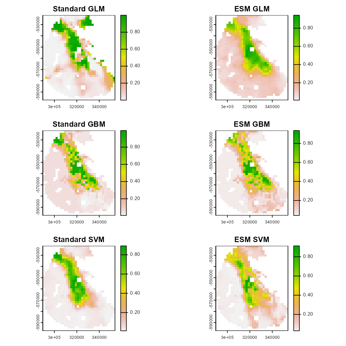
# points(hespero$x, hespero$y, pch = 19)Next, we look at some performance metrics for our models, which are based on our repeated k-folds cross-validation partition method. This can be easily done using the “sdm_summarize()” function in flexsdm. Here, we can see that AUC, TSS, and Jaccard index are higher for the ESMs than their corresponding standard model. However, the Boyce index and the Inverse Mean Absolute Error are slightly higher for the standard models.
merge_df <- sdm_summarize(models = list(mglm, mgbm, msvm, eglm, egbm, esvm))

knitr::kable(
  merge_df %>% dplyr::select(
    model,
    AUC = AUC_mean,
    TSS = TSS_mean,
    JACCARD = JACCARD_mean,
    BOYCE = BOYCE_mean,
    IMAE = IMAE_mean
  )
)| model | AUC | TSS | JACCARD | BOYCE | IMAE |
|---|---|---|---|---|---|
| glm | 0.826575 | 0.694 | 0.7539524 | NA | 0.7484773 |
| gbm | 0.865000 | 0.802 | 0.8219524 | NA | 0.7459401 |
| svm | 0.916600 | 0.862 | 0.8756667 | NA | 0.7214870 |
| esm_glm | 0.884000 | 0.793 | 0.8219524 | NA | 0.7058935 |
| esm_gbm | 0.927725 | 0.846 | 0.8550000 | NA | 0.7461444 |
| esm_svm | 0.936300 | 0.876 | 0.8879524 | NA | 0.7131791 |
Conclusions
Modeling decisions are context-dependent and must be made on a case-by-case basis. However, ESM is a useful approach for practitioners who are interested in modeling very rare species and want to avoid common model overfitting issues. As always when producing SDMs for “real-world” applications, it is important to consider spatial prediction patterns along with multiple model performance metrics.
References
- Lomba, A., L. Pellissier, C. Randin, J. Vicente, F. Moreira, J. Honrado, and A. Guisan. 2010. Overcoming the rare species modelling paradox: A novel hierarchical framework applied to an Iberian endemic plant. Biological conservation 143:2647–2657. https://doi.org/10.1016/j.biocon.2010.07.007
- Breiner, F. T., Guisan, A., Bergamini, A., & Nobis, M. P. (2015). Overcoming limitations of modelling rare species by using ensembles of small models. Methods in Ecology and Evolution, 6(10), 1210–1218. https://doi.org/10.1111/2041-210X.12403
- Breiner, F. T., Nobis, M. P., Bergamini, A., & Guisan, A. (2018). Optimizing ensembles of small models for predicting the distribution of species with few occurrences. Methods in Ecology and Evolution, 9(4), 802–808. https://doi.org/10.1111/2041-210X.12957
- Dubos, N., Montfort, F., Grinand, C., Nourtier, M., Deso, G., Probst, J.-M., Razafimanahaka, J. H., Andriantsimanarilafy, R. R., Rakotondrasoa, E. F., Razafindraibe, P., Jenkins, R., & Crottini, A. (2021). Are narrow-ranging species doomed to extinction? Projected dramatic decline in future climate suitability of two highly threatened species. Perspectives in Ecology and Conservation, S2530064421000894. https://doi.org/10.1016/j.pecon.2021.10.002