Select filtered occurrences based on number of records and spatial autocorrelation (see details)
Arguments
- occ_list
list. A list with filtered specie occurrences testing several values (see
occfilt_envandoccfilt_geo)- x
character. Column name with longitude data
- y
character. Column name with latitude data
- env_layer
SpatRaster. Raster variables that will be used to fit the model. Factor variables will be removed.
- filter_prop
logical. If TRUE, the function will return a list with the filtered occurrences and a tibble with the spatial autocorrelation and number of occurrence values
Value
If filter_prop = FALSE, a tibble with selected filtered occurrences. If filter_prop = TRUE, a list with following objects:
A tibble with selected filtered occurrences
A tibble with filter properties with columns:
filt_value: values used for filtering, the value with an asterisk will denote the one selected
n_records: number of occurrence
mean_autocorr: mean spatial autocorrelation.
the remaining columns have the spatial autocorrelation values for each variable.
Details
The function implement the approach used in Velazco et al. (2020) which consists in calculating for each filtered dataset:
1- the number of occurrence.
2- the spatial autocorrelation based on Morans'I for each variable
3- the mean spatial autocorrelation among variables
Then function will select those dataset with average spatial autocorrelation lower than the mean of all dataset, and from this subset will select the one with the highest number occurrences.
If use occfilt_select cite Velazco et al. (2020) as reference.
References
Velazco, S. J. E., Svenning, J-C., Ribeiro, B. R., & Laureto, L. M. O. (2020). On opportunities and threats to conserve the phylogenetic diversity of Neotropical palms. Diversity and Distributions, 27, 512–523. https://doi.org/10.1111/ddi.13215
Examples
data("spp")
somevar <- terra::rast(system.file("external/somevar.tif", package = "flexsdm"))
sp1 <- spp[spp$species == "sp1" & spp$pr_ab == 1, ]
# Filter records with several coarser resolutions (cell size method)
filtered_occ <- occfilt_geo(
data = sp1,
x = "x",
y = "y",
env_layer = somevar,
method = c("cellsize", factor = c(4, 8, 12)),
prj = terra::crs(somevar)
)
#> Extracting values from raster ...
#> 16 records were removed because they have NAs for some variables
#> Number of unfiltered records: 234
#> Factor: x4
#> Distance threshold (km): 6.157
#> Number of filtered records: 203
#> Factor: x8
#> Distance threshold (km): 12.313
#> Number of filtered records: 156
#> Factor: x12
#> Distance threshold (km): 18.47
#> Number of filtered records: 117
# Select the filtered data based on number of records and spatial autocorrelation
occ_selected <- occfilt_select(
occ_list = filtered_occ,
x = "x",
y = "y",
env_layer = somevar,
filter_prop = FALSE
)
#> Dataset with filtered value 12 was selected
nrow(occ_selected)
#> [1] 117
# \donttest{
require(terra)
require(dplyr)
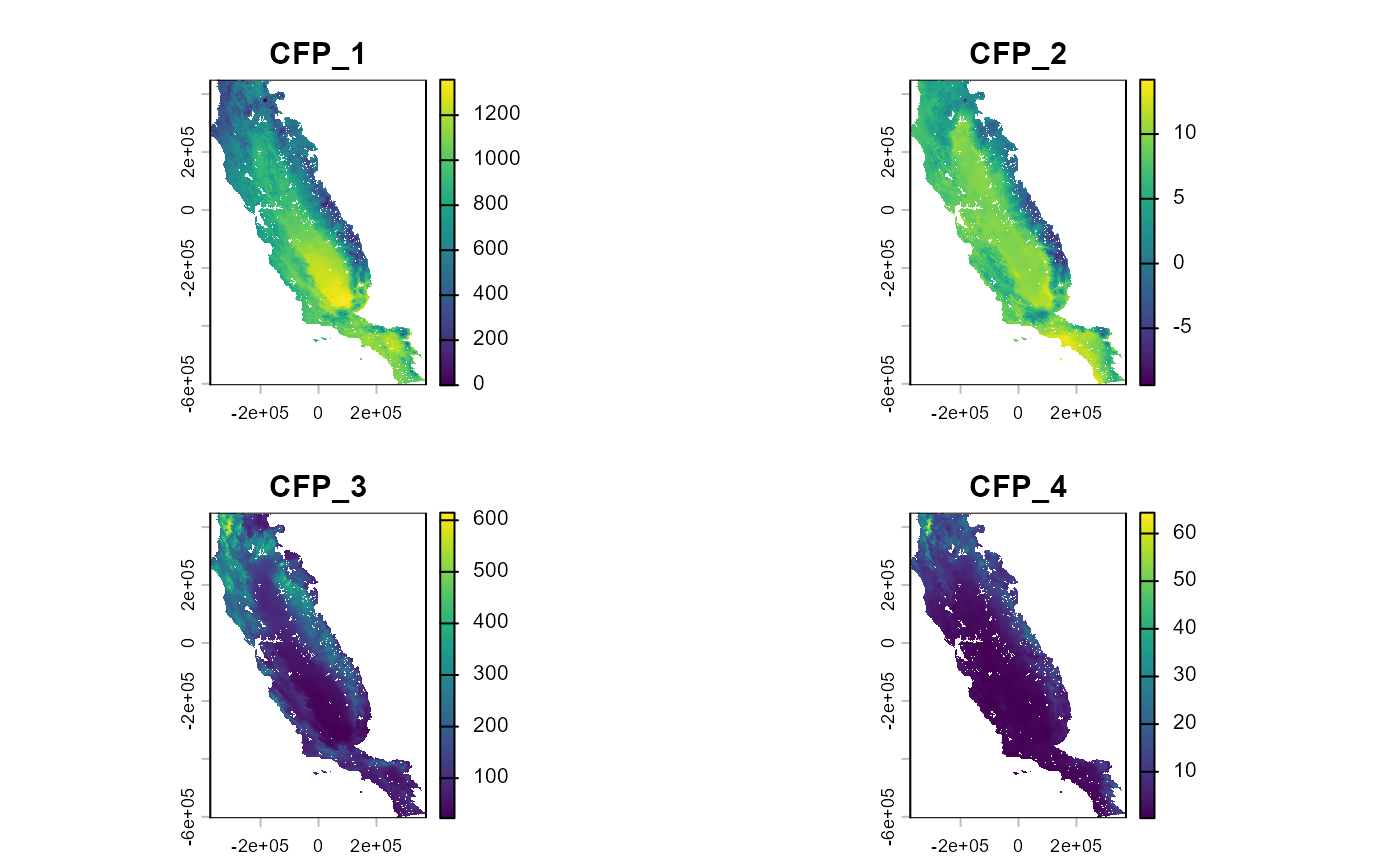
# Environmental variables
somevar <- system.file("external/somevar.tif", package = "flexsdm")
somevar <- terra::rast(somevar)
plot(somevar)
 # Species occurrences
data("spp")
spp
#> # A tibble: 1,150 × 4
#> species x y pr_ab
#> <chr> <dbl> <dbl> <dbl>
#> 1 sp1 -5541. -145138. 0
#> 2 sp1 -51981. 16322. 0
#> 3 sp1 -269871. 69512. 1
#> 4 sp1 -96261. -32008. 0
#> 5 sp1 269589. -566338. 0
#> 6 sp1 29829. -328468. 0
#> 7 sp1 -152691. 393782. 0
#> 8 sp1 -195081. 253652. 0
#> 9 sp1 -951. -277978. 0
#> 10 sp1 145929. -271498. 0
#> # ℹ 1,140 more rows
spp1 <- spp %>% dplyr::filter(species == "sp1", pr_ab == 1)
## %######################################################%##
#### Cellsize method ####
## %######################################################%##
# Using cellsize method
filtered_occ <- occfilt_geo(
data = spp1,
x = "x",
y = "y",
env_layer = somevar,
method = c("cellsize", factor = c(1, 4, 8, 12, 16, 20)),
prj = crs(somevar)
)
#> Extracting values from raster ...
#> 16 records were removed because they have NAs for some variables
#> Number of unfiltered records: 234
#> Factor: x1
#> Distance threshold (km): 1.539
#> Number of filtered records: 233
#> Factor: x4
#> Distance threshold (km): 6.157
#> Number of filtered records: 203
#> Factor: x8
#> Distance threshold (km): 12.313
#> Number of filtered records: 156
#> Factor: x12
#> Distance threshold (km): 18.47
#> Number of filtered records: 118
#> Factor: x16
#> Distance threshold (km): 24.626
#> Number of filtered records: 96
#> Factor: x20
#> Distance threshold (km): 30.783
#> Number of filtered records: 78
filtered_occ
#> $`1`
#> # A tibble: 233 × 4
#> species x y pr_ab
#> <chr> <dbl> <dbl> <dbl>
#> 1 sp1 -269871. 69512. 1
#> 2 sp1 -149991. 267962. 1
#> 3 sp1 -126231. 196142. 1
#> 4 sp1 91659. -156748. 1
#> 5 sp1 -210471. 326282. 1
#> 6 sp1 -140541. 284972. 1
#> 7 sp1 -217491. 65732. 1
#> 8 sp1 -178611. 225032. 1
#> 9 sp1 -92481. 155642. 1
#> 10 sp1 -367611. 266072. 1
#> # ℹ 223 more rows
#>
#> $`4`
#> # A tibble: 203 × 4
#> species x y pr_ab
#> <chr> <dbl> <dbl> <dbl>
#> 1 sp1 -269871. 69512. 1
#> 2 sp1 -149991. 267962. 1
#> 3 sp1 -126231. 196142. 1
#> 4 sp1 91659. -156748. 1
#> 5 sp1 -210471. 326282. 1
#> 6 sp1 -140541. 284972. 1
#> 7 sp1 -217491. 65732. 1
#> 8 sp1 -178611. 225032. 1
#> 9 sp1 -92481. 155642. 1
#> 10 sp1 -367611. 266072. 1
#> # ℹ 193 more rows
#>
#> $`8`
#> # A tibble: 156 × 4
#> species x y pr_ab
#> <chr> <dbl> <dbl> <dbl>
#> 1 sp1 -269871. 69512. 1
#> 2 sp1 -149991. 267962. 1
#> 3 sp1 91659. -156748. 1
#> 4 sp1 -210471. 326282. 1
#> 5 sp1 -140541. 284972. 1
#> 6 sp1 -217491. 65732. 1
#> 7 sp1 -92481. 155642. 1
#> 8 sp1 -367611. 266072. 1
#> 9 sp1 -109491. 46292. 1
#> 10 sp1 -260151. 57632. 1
#> # ℹ 146 more rows
#>
#> $`12`
#> # A tibble: 118 × 4
#> species x y pr_ab
#> <chr> <dbl> <dbl> <dbl>
#> 1 sp1 -269871. 69512. 1
#> 2 sp1 -140541. 284972. 1
#> 3 sp1 -178611. 225032. 1
#> 4 sp1 -34431. 212072. 1
#> 5 sp1 -215871. -51178. 1
#> 6 sp1 -60351. -307138. 1
#> 7 sp1 -331161. 387842. 1
#> 8 sp1 -88971. 137282. 1
#> 9 sp1 -120021. 110282. 1
#> 10 sp1 -195351. 85982. 1
#> # ℹ 108 more rows
#>
#> $`16`
#> # A tibble: 96 × 4
#> species x y pr_ab
#> <chr> <dbl> <dbl> <dbl>
#> 1 sp1 -210471. 326282. 1
#> 2 sp1 -140541. 284972. 1
#> 3 sp1 -313611. 400802. 1
#> 4 sp1 -202911. -64138. 1
#> 5 sp1 -34431. 212072. 1
#> 6 sp1 -172941. -113008. 1
#> 7 sp1 -60351. -307138. 1
#> 8 sp1 -148911. 247712. 1
#> 9 sp1 -195351. 85982. 1
#> 10 sp1 -23091. 56012. 1
#> # ℹ 86 more rows
#>
#> $`20`
#> # A tibble: 78 × 4
#> species x y pr_ab
#> <chr> <dbl> <dbl> <dbl>
#> 1 sp1 -210471. 326282. 1
#> 2 sp1 -178611. 225032. 1
#> 3 sp1 -367611. 266072. 1
#> 4 sp1 -34431. 212072. 1
#> 5 sp1 -143781. 233942. 1
#> 6 sp1 -215871. -51178. 1
#> 7 sp1 -60351. -307138. 1
#> 8 sp1 -195351. 85982. 1
#> 9 sp1 -328731. 405392. 1
#> 10 sp1 -114621. 54122. 1
#> # ℹ 68 more rows
#>
# Select filtered occurrences based on
# number of records and spatial autocorrelation
occ_selected <- occfilt_select(
occ_list = filtered_occ,
x = "x",
y = "y",
env_layer = somevar,
filter_prop = FALSE
)
#> Dataset with filtered value 12 was selected
occ_selected
#> # A tibble: 118 × 4
#> species x y pr_ab
#> <chr> <dbl> <dbl> <dbl>
#> 1 sp1 -269871. 69512. 1
#> 2 sp1 -140541. 284972. 1
#> 3 sp1 -178611. 225032. 1
#> 4 sp1 -34431. 212072. 1
#> 5 sp1 -215871. -51178. 1
#> 6 sp1 -60351. -307138. 1
#> 7 sp1 -331161. 387842. 1
#> 8 sp1 -88971. 137282. 1
#> 9 sp1 -120021. 110282. 1
#> 10 sp1 -195351. 85982. 1
#> # ℹ 108 more rows
occ_selected <- occfilt_select(
occ_list = filtered_occ,
x = "x",
y = "y",
env_layer = somevar,
filter_prop = TRUE
)
#> Dataset with filtered value 12 was selected
occ_selected$occ
#> # A tibble: 118 × 4
#> species x y pr_ab
#> <chr> <dbl> <dbl> <dbl>
#> 1 sp1 -269871. 69512. 1
#> 2 sp1 -140541. 284972. 1
#> 3 sp1 -178611. 225032. 1
#> 4 sp1 -34431. 212072. 1
#> 5 sp1 -215871. -51178. 1
#> 6 sp1 -60351. -307138. 1
#> 7 sp1 -331161. 387842. 1
#> 8 sp1 -88971. 137282. 1
#> 9 sp1 -120021. 110282. 1
#> 10 sp1 -195351. 85982. 1
#> # ℹ 108 more rows
occ_selected$filter_prop
#> filt_value mean_autocorr n_records CFP_1 CFP_2 CFP_3 CFP_4
#> 1 1 0.3219265 233 0.3534014 0.20178498 0.3352363 0.3972832
#> 2 4 0.2883075 203 0.3192020 0.15468048 0.3059884 0.3733591
#> 3 8 0.2612257 156 0.3024255 0.12227197 0.2771447 0.3430608
#> 4 * 12 0.2317656 118 0.2642331 0.11277701 0.2303653 0.3196870
#> 5 16 0.2169756 96 0.2713333 0.07524462 0.2383771 0.2829474
#> 6 20 0.2015422 78 0.2381032 0.07769944 0.2004469 0.2899193
# }
# Species occurrences
data("spp")
spp
#> # A tibble: 1,150 × 4
#> species x y pr_ab
#> <chr> <dbl> <dbl> <dbl>
#> 1 sp1 -5541. -145138. 0
#> 2 sp1 -51981. 16322. 0
#> 3 sp1 -269871. 69512. 1
#> 4 sp1 -96261. -32008. 0
#> 5 sp1 269589. -566338. 0
#> 6 sp1 29829. -328468. 0
#> 7 sp1 -152691. 393782. 0
#> 8 sp1 -195081. 253652. 0
#> 9 sp1 -951. -277978. 0
#> 10 sp1 145929. -271498. 0
#> # ℹ 1,140 more rows
spp1 <- spp %>% dplyr::filter(species == "sp1", pr_ab == 1)
## %######################################################%##
#### Cellsize method ####
## %######################################################%##
# Using cellsize method
filtered_occ <- occfilt_geo(
data = spp1,
x = "x",
y = "y",
env_layer = somevar,
method = c("cellsize", factor = c(1, 4, 8, 12, 16, 20)),
prj = crs(somevar)
)
#> Extracting values from raster ...
#> 16 records were removed because they have NAs for some variables
#> Number of unfiltered records: 234
#> Factor: x1
#> Distance threshold (km): 1.539
#> Number of filtered records: 233
#> Factor: x4
#> Distance threshold (km): 6.157
#> Number of filtered records: 203
#> Factor: x8
#> Distance threshold (km): 12.313
#> Number of filtered records: 156
#> Factor: x12
#> Distance threshold (km): 18.47
#> Number of filtered records: 118
#> Factor: x16
#> Distance threshold (km): 24.626
#> Number of filtered records: 96
#> Factor: x20
#> Distance threshold (km): 30.783
#> Number of filtered records: 78
filtered_occ
#> $`1`
#> # A tibble: 233 × 4
#> species x y pr_ab
#> <chr> <dbl> <dbl> <dbl>
#> 1 sp1 -269871. 69512. 1
#> 2 sp1 -149991. 267962. 1
#> 3 sp1 -126231. 196142. 1
#> 4 sp1 91659. -156748. 1
#> 5 sp1 -210471. 326282. 1
#> 6 sp1 -140541. 284972. 1
#> 7 sp1 -217491. 65732. 1
#> 8 sp1 -178611. 225032. 1
#> 9 sp1 -92481. 155642. 1
#> 10 sp1 -367611. 266072. 1
#> # ℹ 223 more rows
#>
#> $`4`
#> # A tibble: 203 × 4
#> species x y pr_ab
#> <chr> <dbl> <dbl> <dbl>
#> 1 sp1 -269871. 69512. 1
#> 2 sp1 -149991. 267962. 1
#> 3 sp1 -126231. 196142. 1
#> 4 sp1 91659. -156748. 1
#> 5 sp1 -210471. 326282. 1
#> 6 sp1 -140541. 284972. 1
#> 7 sp1 -217491. 65732. 1
#> 8 sp1 -178611. 225032. 1
#> 9 sp1 -92481. 155642. 1
#> 10 sp1 -367611. 266072. 1
#> # ℹ 193 more rows
#>
#> $`8`
#> # A tibble: 156 × 4
#> species x y pr_ab
#> <chr> <dbl> <dbl> <dbl>
#> 1 sp1 -269871. 69512. 1
#> 2 sp1 -149991. 267962. 1
#> 3 sp1 91659. -156748. 1
#> 4 sp1 -210471. 326282. 1
#> 5 sp1 -140541. 284972. 1
#> 6 sp1 -217491. 65732. 1
#> 7 sp1 -92481. 155642. 1
#> 8 sp1 -367611. 266072. 1
#> 9 sp1 -109491. 46292. 1
#> 10 sp1 -260151. 57632. 1
#> # ℹ 146 more rows
#>
#> $`12`
#> # A tibble: 118 × 4
#> species x y pr_ab
#> <chr> <dbl> <dbl> <dbl>
#> 1 sp1 -269871. 69512. 1
#> 2 sp1 -140541. 284972. 1
#> 3 sp1 -178611. 225032. 1
#> 4 sp1 -34431. 212072. 1
#> 5 sp1 -215871. -51178. 1
#> 6 sp1 -60351. -307138. 1
#> 7 sp1 -331161. 387842. 1
#> 8 sp1 -88971. 137282. 1
#> 9 sp1 -120021. 110282. 1
#> 10 sp1 -195351. 85982. 1
#> # ℹ 108 more rows
#>
#> $`16`
#> # A tibble: 96 × 4
#> species x y pr_ab
#> <chr> <dbl> <dbl> <dbl>
#> 1 sp1 -210471. 326282. 1
#> 2 sp1 -140541. 284972. 1
#> 3 sp1 -313611. 400802. 1
#> 4 sp1 -202911. -64138. 1
#> 5 sp1 -34431. 212072. 1
#> 6 sp1 -172941. -113008. 1
#> 7 sp1 -60351. -307138. 1
#> 8 sp1 -148911. 247712. 1
#> 9 sp1 -195351. 85982. 1
#> 10 sp1 -23091. 56012. 1
#> # ℹ 86 more rows
#>
#> $`20`
#> # A tibble: 78 × 4
#> species x y pr_ab
#> <chr> <dbl> <dbl> <dbl>
#> 1 sp1 -210471. 326282. 1
#> 2 sp1 -178611. 225032. 1
#> 3 sp1 -367611. 266072. 1
#> 4 sp1 -34431. 212072. 1
#> 5 sp1 -143781. 233942. 1
#> 6 sp1 -215871. -51178. 1
#> 7 sp1 -60351. -307138. 1
#> 8 sp1 -195351. 85982. 1
#> 9 sp1 -328731. 405392. 1
#> 10 sp1 -114621. 54122. 1
#> # ℹ 68 more rows
#>
# Select filtered occurrences based on
# number of records and spatial autocorrelation
occ_selected <- occfilt_select(
occ_list = filtered_occ,
x = "x",
y = "y",
env_layer = somevar,
filter_prop = FALSE
)
#> Dataset with filtered value 12 was selected
occ_selected
#> # A tibble: 118 × 4
#> species x y pr_ab
#> <chr> <dbl> <dbl> <dbl>
#> 1 sp1 -269871. 69512. 1
#> 2 sp1 -140541. 284972. 1
#> 3 sp1 -178611. 225032. 1
#> 4 sp1 -34431. 212072. 1
#> 5 sp1 -215871. -51178. 1
#> 6 sp1 -60351. -307138. 1
#> 7 sp1 -331161. 387842. 1
#> 8 sp1 -88971. 137282. 1
#> 9 sp1 -120021. 110282. 1
#> 10 sp1 -195351. 85982. 1
#> # ℹ 108 more rows
occ_selected <- occfilt_select(
occ_list = filtered_occ,
x = "x",
y = "y",
env_layer = somevar,
filter_prop = TRUE
)
#> Dataset with filtered value 12 was selected
occ_selected$occ
#> # A tibble: 118 × 4
#> species x y pr_ab
#> <chr> <dbl> <dbl> <dbl>
#> 1 sp1 -269871. 69512. 1
#> 2 sp1 -140541. 284972. 1
#> 3 sp1 -178611. 225032. 1
#> 4 sp1 -34431. 212072. 1
#> 5 sp1 -215871. -51178. 1
#> 6 sp1 -60351. -307138. 1
#> 7 sp1 -331161. 387842. 1
#> 8 sp1 -88971. 137282. 1
#> 9 sp1 -120021. 110282. 1
#> 10 sp1 -195351. 85982. 1
#> # ℹ 108 more rows
occ_selected$filter_prop
#> filt_value mean_autocorr n_records CFP_1 CFP_2 CFP_3 CFP_4
#> 1 1 0.3219265 233 0.3534014 0.20178498 0.3352363 0.3972832
#> 2 4 0.2883075 203 0.3192020 0.15468048 0.3059884 0.3733591
#> 3 8 0.2612257 156 0.3024255 0.12227197 0.2771447 0.3430608
#> 4 * 12 0.2317656 118 0.2642331 0.11277701 0.2303653 0.3196870
#> 5 16 0.2169756 96 0.2713333 0.07524462 0.2383771 0.2829474
#> 6 20 0.2015422 78 0.2381032 0.07769944 0.2004469 0.2899193
# }