vignettes/v04_Red_fir_example.Rmd
v04_Red_fir_example.Rmdtitle: ‘flexsdm: Red Fir example’ output: rmarkdown::html_vignette vignette: > % % % —
Example of full modeling process
Study species & overview of methods
Here, we used the flexsdm package to model the current distribution of California red fir (Abies magnifica). Red fir is a high-elevation conifer species that’s geographic range extends through the Sierra Nevada in California, USA, into the southern portion of the Cascade Range of Oregon. For this species, we used presence data compiled from several public datasets curated by natural resources agencies. We built the distribution models using four hydro-climatic variables: actual evapotranspiration, climatic water deficit, maximum temperature of the warmest month, and minimum temperature of the coldest month. All variables were resampled (aggregated) to a 1890 m spatial resolution to improve processing time.
Delimit of a calibration area
Delimiting the calibration area (aka accessible area) is an essential step in SDMs both in methodological and theoretical terms. The calibration area will affect several characteristics of a SDM like the range of environmental variables, the number of absences, the distribution of background points and pseudo-absences, and unfortunately, some performance metrics like AUC and TSS. There are several ways to delimit a calibration area. In calib_area(). We used a method that the calibration area is delimited by a 100-km buffer around presences (shown in the figure below).
# devtools::install_github('sjevelazco/flexsdm')
library(flexsdm)
library(terra)
library(dplyr)

somevar <- system.file("external/somevar.tif", package = "flexsdm")
somevar <- terra::rast(somevar) # environmental data
names(somevar) <- c("aet", "cwd", "tmx", "tmn")
data(abies)
abies_p <- abies %>%
  select(x, y, pr_ab) %>%
  filter(pr_ab == 1) # filter only for presence locations

ca <-
  calib_area(
    data = abies_p,
    x = "x",
    y = "y",
    method = c("buffer", width = 100000),
    crs = crs(somevar)
  ) # create a calibration area with 100 km buffer around occurrence points

# visualize the species occurrences
layer1 <- somevar[[1]]
layer1[!is.na(layer1)] <- 1

plot(layer1, col = "gray80", legend = FALSE, axes = FALSE)
plot(crop(ca, layer1), add = TRUE)
points(abies_p[, c("x", "y")], col = "#00000480")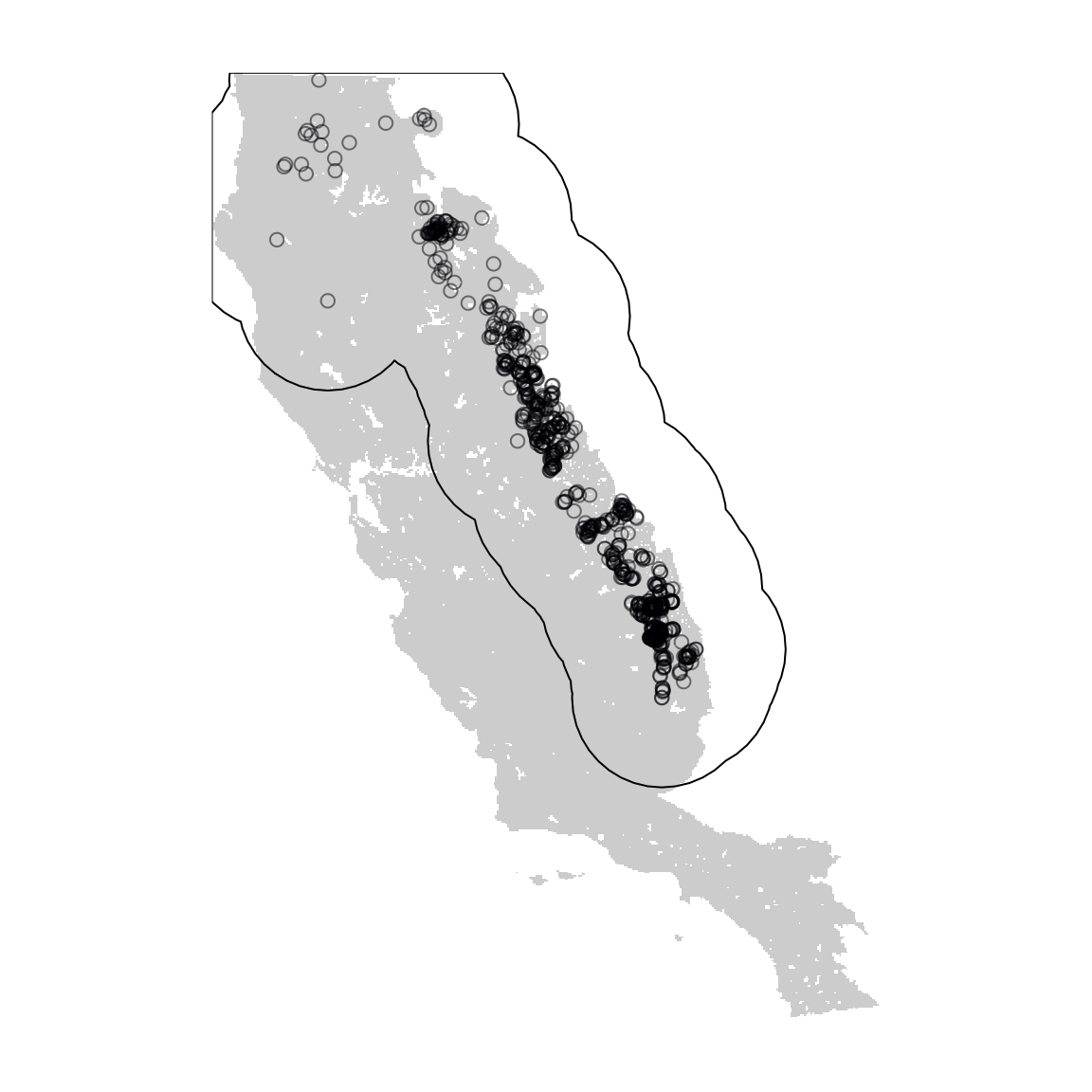
Occurrence filtering
Sample bias in species occurrence data has long been a recognized issue in SDM. However, environmental filtering of observation data can improve model predictions by reducing redundancy in environmental (e.g. climatic) hyper-space (Varela et al. 2014). Here we will use the function occfilt_env() to thin the red fir occurrences based on environmental space. This function is unique to flexsdm, and in contrast with other packages is able to use any number of environmental dimensions and does not perform a PCA before filtering.
Next we apply environmental occurrence filtering using 8 bins and display the resulting filtered occurrence data
abies_p$id <- 1:nrow(abies_p) # adding unique id to each row
abies_pf <- abies_p %>%
  occfilt_env(
    data = .,
    x = "x",
    y = "y",
    id = "id",
    nbins = 8,
    env_layer = somevar
  ) %>%
  left_join(abies_p, by = c("id", "x", "y"))
#> Extracting values from raster ...
#> 27 records were removed because they have NAs for some variables
#> Number of unfiltered records: 673
#> Number of filtered records: 216

plot(layer1, col = "gray80", legend = FALSE, axes = FALSE)
plot(crop(ca, layer1), add = TRUE)
points(abies_p[, c("x", "y")], col = "#00000480")
points(abies_pf[, c("x", "y")], col = "#5DC86180")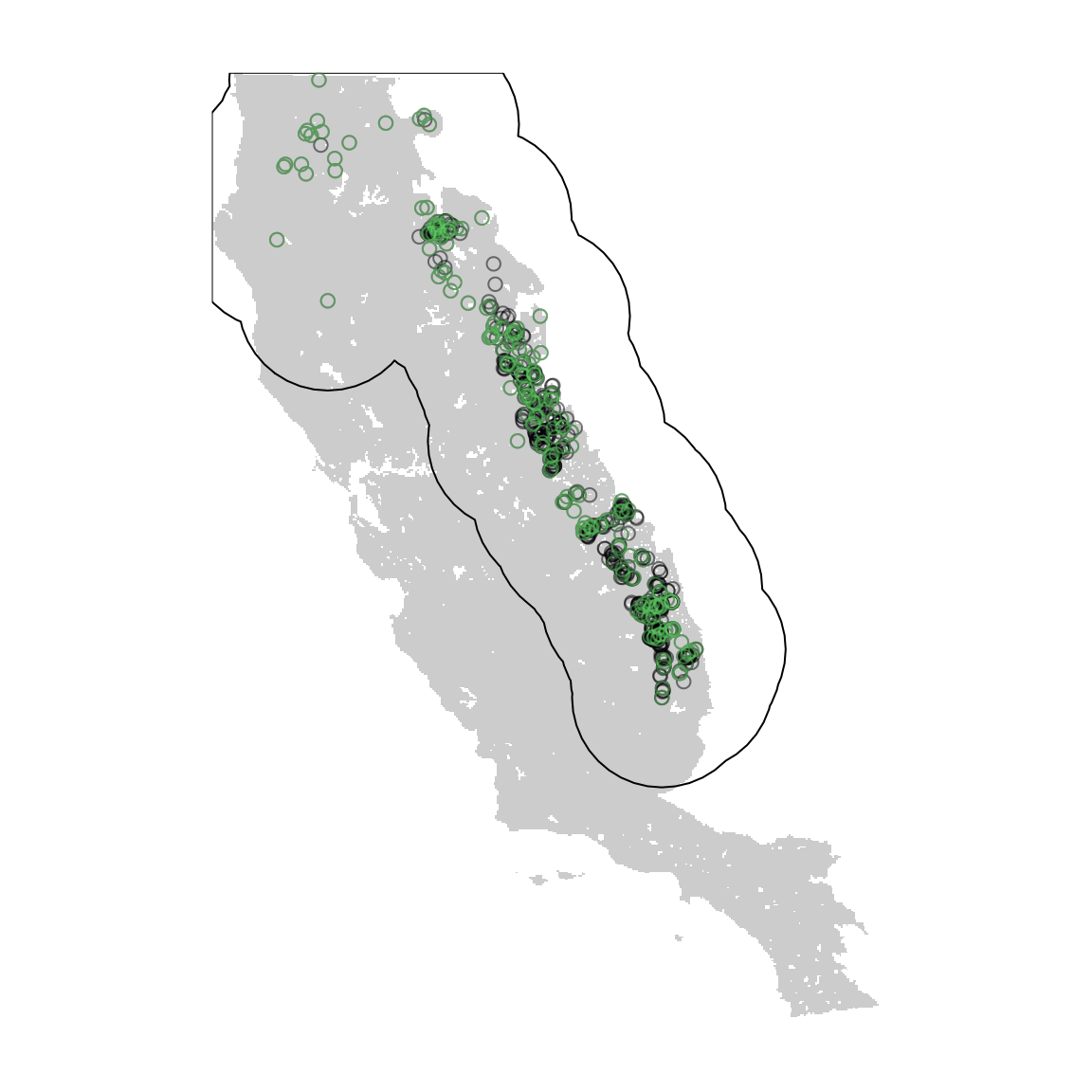
Block partition with 4 folds
Data partitioning, or splitting data into testing and training groups, is a key step in building SDMs. flexsdm offers multiple options for data partitioning and here we use a spatial block method. Geographically structured data partitioning methods are especially useful if users want to evaluate model transferability to different regions or time periods. The part_sblock() function explores spatial blocks with different raster cells sizes and returns the one that is best suited for the input datset based on spatial autocorrelation, environmental similarity, and the number of presence/absence records in each block partition. The function’s output provides users with 1) a tibble with presence/absence locations and the assigned partition number, 2) a tibble with information about the best partition, and 3) a SpatRaster showing the selected grid. Here we want to divide the data into 4 different partitions using the spatial block method.
set.seed(10)
occ_part <- abies_pf %>%
  part_sblock(
    data = .,
    env_layer = somevar,
    pr_ab = "pr_ab",
    x = "x",
    y = "y",
    n_part = 4,
    min_res_mult = 3,
    max_res_mult = 200,
    num_grids = 30,
    prop = 1
  )
#> The following grid cell sizes will be tested:
#> 5670 | 18508.97 | 31347.93 | 44186.9 | 57025.86 | 69864.83 | 82703.79 | 95542.76 | 108381.72 | 121220.69 | 134059.66 | 146898.62 | 159737.59 | 172576.55 | 185415.52 | 198254.48 | 211093.45 | 223932.41 | 236771.38 | 249610.34 | 262449.31 | 275288.28 | 288127.24 | 300966.21 | 313805.17 | 326644.14 | 339483.1 | 352322.07 | 365161.03 | 378000
#> Creating basic raster mask...
#> Searching for the optimal grid size...
abies_pf <- occ_part$part

# Transform best block partition to a raster layer with same resolution and extent than
# predictor variables
block_layer <- get_block(env_layer = somevar, best_grid = occ_part$grid)

cl <- c("#64146D", "#9E2962", "#F47C15", "#FCFFA4")
plot(block_layer, col = cl, legend = FALSE, axes = FALSE)
points(abies_pf[, c("x", "y")])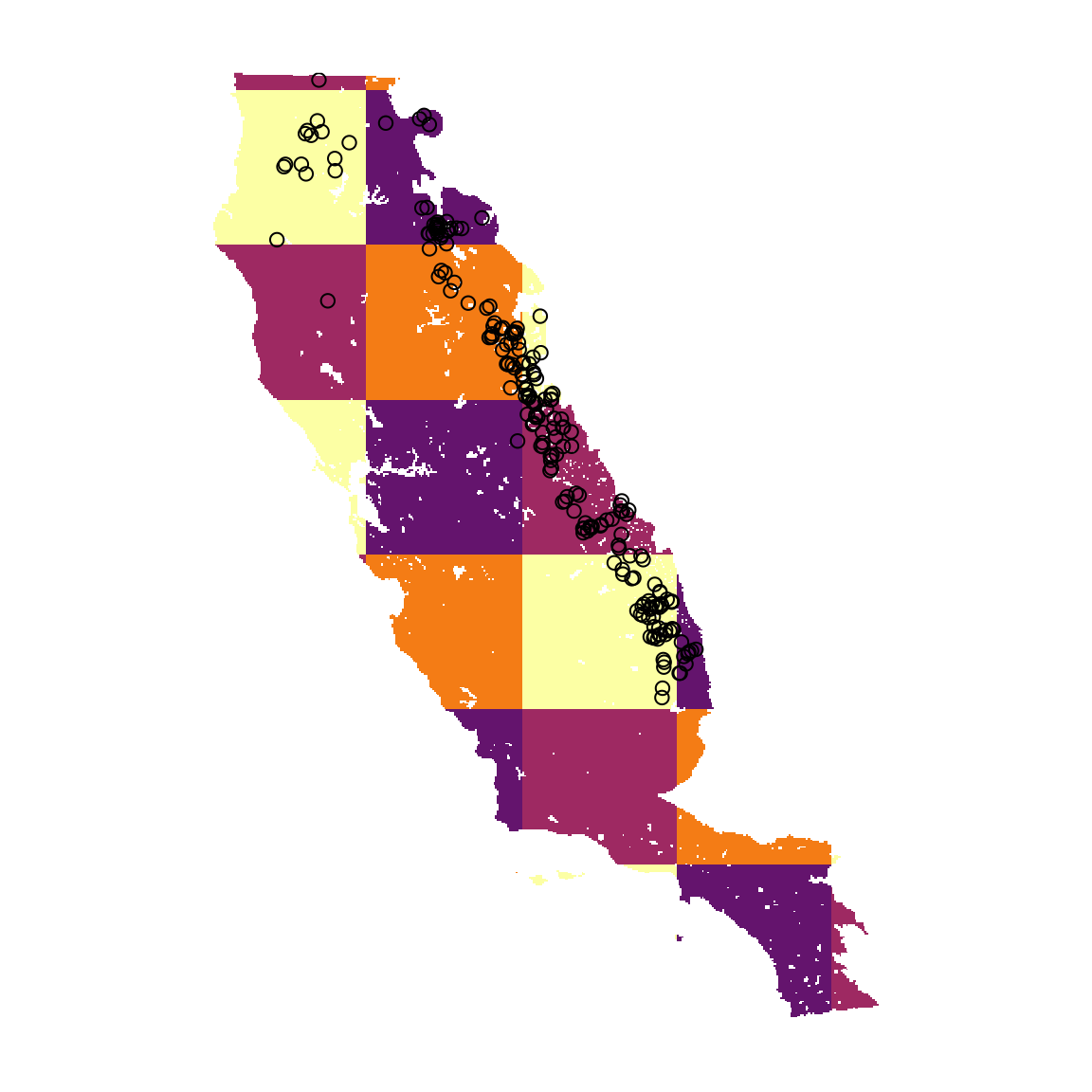
# Number of presences per block
abies_pf %>%
  dplyr::group_by(.part) %>%
  dplyr::count()
#> # A tibble: 4 × 2
#> # Groups:   .part [4]
#>   .part     n
#>   <int> <int>
#> 1     1    38
#> 2     2    59
#> 3     3    33
#> 4     4    86
# Additional information of the best block
occ_part$best_part_info
#> # A tibble: 1 × 5
#>   n_grid cell_size spa_auto env_sim  sd_p
#>    <int>     <dbl>    <dbl>   <dbl> <dbl>
#> 1     14   172577.      0.5    173.  24.1
Pseudo-absence/background points (using partition previously created as a mask)
In this example, we only have species presence data. However, most SDM methods require either pseudo-absence or background data. Here, we will use the spatial block partition we just created to generate pseudo-absence and background points.
# Spatial blocks where species occurs
# Sample background points throughout study area with random method, allocating 10X the number of presences a background
set.seed(10)
bg <- lapply(1:4, function(x) {
  sample_background(
    data = abies_pf,
    x = "x",
    y = "y",
    n = sum(abies_pf$.part == x) * 10,
    method = "random",
    rlayer = block_layer,
    maskval = x,
    calibarea = ca
  )
}) %>%
  bind_rows()
bg <- sdm_extract(data = bg, x = "x", y = "y", env_layer = block_layer)

# Sample a number of pseudo-absences equal to the presence in each partition
set.seed(10)
psa <- lapply(1:4, function(x) {
  sample_pseudoabs(
    data = abies_pf,
    x = "x",
    y = "y",
    n = sum(abies_pf$.part == x),
    method = "random",
    rlayer = block_layer,
    maskval = x,
    calibarea = ca
  )
}) %>%
  bind_rows()
psa <- sdm_extract(data = psa, x = "x", y = "y", env_layer = block_layer)

cl <- c("#280B50", "#9E2962", "#F47C15", "#FCFFA4")
plot(block_layer, col = "gray80", legend = FALSE, axes = FALSE)
points(bg[, c("x", "y")], col = cl[bg$.part], cex = 0.8) # Background points
points(psa[, c("x", "y")], bg = cl[psa$.part], cex = 0.8, pch = 21) # Pseudo-absences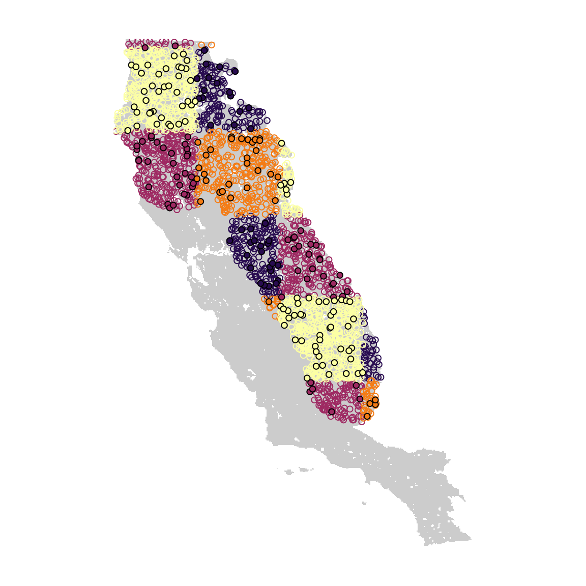
# Bind a presences and pseudo-absences
abies_pa <- bind_rows(abies_pf, psa)
abies_pa # Presence-Pseudo-absence database
#> # A tibble: 432 × 4
#>          x        y pr_ab .part
#>      <dbl>    <dbl> <dbl> <dbl>
#>  1 -12558.   68530.     1     2
#>  2 115217. -145937.     1     4
#>  3   3634.   22501.     1     2
#>  4  44972.  -60781.     1     2
#>  5 -34463.  160313.     1     3
#>  6  83108.  -27300.     1     2
#>  7 124877. -176319.     1     4
#>  8 118707. -179991.     1     4
#>  9 126141. -176302.     1     4
#> 10 -49722.  141124.     1     3
#> # ℹ 422 more rows
bg # Background points
#> # A tibble: 2,160 × 4
#>           x       y pr_ab .part
#>       <dbl>   <dbl> <dbl> <dbl>
#>  1 -153501. 392162.     0     1
#>  2  -89241. 263642.     0     1
#>  3  -89241.  27392.     0     1
#>  4 -130821. 331682.     0     1
#>  5 -132711. 339242.     0     1
#>  6  -51441. -63328.     0     1
#>  7  -59001.  67082.     0     1
#>  8  -32541. -51988.     0     1
#>  9  -96801.    932.     0     1
#> 10  -47661. -31198.     0     1
#> # ℹ 2,150 more rows
Extract environmental data for the presence-absence and background data . View the distributions of present points, pseudo-absence points, and background points using the blocks as a reference map.
abies_pa <- abies_pa %>%
  sdm_extract(
    data = .,
    x = "x",
    y = "y",
    env_layer = somevar,
    filter_na = TRUE
  )
bg <- bg %>%
  sdm_extract(
    data = .,
    x = "x",
    y = "y",
    env_layer = somevar,
    filter_na = TRUE
  )
Fit models with tune_max, fit_gau, and fit_glm
Now, fit our models. The flexsdm package offers a wide range of modeling options, from traditional statistical methods like GLMs and GAMs, to machine learning methods like random forests and support vector machines. For each modeling method, flexsdm provides both fit_ and tune_ functions, which allow users to use default settings or adjust hyperparameters depending on their research goals. Here, we will test out tune_max() (tuned Maximum Entropy model), fit_gau() (fit Guassian Process model), and fit_glm (fit Generalized Linear Model). For each model, we selected three threshold values to generate binary suitability predictions: the threshold that maximizes TSS (max_sens_spec), the threshold at which sensitivity and specificity are equal (equal_sens_spec), and the threshold at which the Sorenson index is highest (max_sorenson). In this example, we selected TSS as the performance metric used for selecting the best combination of hyper-parameter values in the tuned Maximum Entropy model.
t_max <- tune_max(
  data = abies_pa,
  response = "pr_ab",
  predictors = names(somevar),
  background = bg,
  partition = ".part",
  grid = expand.grid(
    regmult = seq(0.1, 3, 0.5),
    classes = c("l", "lq", "lqhpt")
  ),
  thr = c("max_sens_spec", "equal_sens_spec", "max_sorensen"),
  metric = "TSS",
  clamp = TRUE,
  pred_type = "cloglog"
)
#> Tuning model...
#> Replica number: 1/1
#> Partition number: 1/4
#> Partition number: 2/4
#> Partition number: 3/4
#> Partition number: 4/4
#> Fitting best model
#> Formula used for model fitting:
#> ~aet + cwd + tmx + tmn + I(aet^2) + I(cwd^2) + I(tmx^2) + I(tmn^2) + hinge(aet) + hinge(cwd) + hinge(tmx) + hinge(tmn) + thresholds(aet) + thresholds(cwd) + thresholds(tmx) + thresholds(tmn) + cwd:aet + tmx:aet + tmn:aet + tmx:cwd + tmn:cwd + tmn:tmx - 1
#> Replica number: 1/1
#> Partition number: 1/4
#> Partition number: 2/4
#> Partition number: 3/4
#> Partition number: 4/4
f_gau <- fit_gau(
  data = abies_pa,
  response = "pr_ab",
  predictors = names(somevar),
  partition = ".part",
  thr = c("max_sens_spec", "equal_sens_spec", "max_sorensen")
)
#> Replica number: 1/1
#> Partition number: 1/4
#> Partition number: 2/4
#> Partition number: 3/4
#> Partition number: 4/4
f_glm <- fit_glm(
  data = abies_pa,
  response = "pr_ab",
  predictors = names(somevar),
  partition = ".part",
  thr = c("max_sens_spec", "equal_sens_spec", "max_sorensen"),
  poly = 2
)
#> Formula used for model fitting:
#> pr_ab ~ aet + cwd + tmx + tmn + I(aet^2) + I(cwd^2) + I(tmx^2) + I(tmn^2)
#> Replica number: 1/1
#> Partition number: 1/4
#> Partition number: 2/4
#> Partition number: 3/4
#> Partition number: 4/4
Fit an ensemble model
Spatial predictions from different SDM algorithms can vary substantially, and ensemble modeling has become increasingly popular. With the fit_ensemble() function, users can easily produce an ensemble SDM based on any of the individual fit_ and tune_ models included the package. In this example, we fit an ensemble model for red fir based on the weighted average of the three individual models. We used the same threshold values and performance metric that were implemented in the individual models.
ens_m <- fit_ensemble(
  models = list(t_max, f_gau, f_glm),
  ens_method = "meanw",
  thr = c("max_sens_spec", "equal_sens_spec", "max_sorensen"),
  thr_model = "max_sens_spec",
  metric = "TSS"
)
#>   |                                                                              |                                                                      |   0%  |                                                                              |======================================================================| 100%
ens_m$performance
#> # A tibble: 3 × 33
#>   model threshold      thr_value n_presences n_absences TPR_mean TPR_sd TNR_mean
#>   <chr> <chr>              <dbl>       <int>      <int>    <dbl>  <dbl>    <dbl>
#> 1 meanw equal_sens_sp…     0.583         216        216    0.794 0.0890    0.794
#> 2 meanw max_sens_spec      0.514         216        216    0.943 0.0262    0.757
#> 3 meanw max_sorensen       0.449         216        216    0.963 0.0143    0.738
#> # ℹ 25 more variables: TNR_sd <dbl>, W_TPR_TNR_mean <dbl>, W_TPR_TNR_sd <dbl>,
#> #   SORENSEN_mean <dbl>, SORENSEN_sd <dbl>, JACCARD_mean <dbl>,
#> #   JACCARD_sd <dbl>, FPB_mean <dbl>, FPB_sd <dbl>, OR_mean <dbl>, OR_sd <dbl>,
#> #   TSS_mean <dbl>, TSS_sd <dbl>, KAPPA_mean <dbl>, KAPPA_sd <dbl>,
#> #   MCC_mean <dbl>, MCC_sd <dbl>, AUC_mean <dbl>, AUC_sd <dbl>,
#> #   BOYCE_mean <dbl>, BOYCE_sd <dbl>, CRPS_mean <dbl>, CRPS_sd <dbl>,
#> #   IMAE_mean <dbl>, IMAE_sd <dbl>
The output of flexsdm model objects allows you to easily compare metrics across models, such as AUC or TSS. For example, we can use the sdm_summarize() function to merge model performance tables.
model_perf <- sdm_summarize(list(t_max, f_gau, f_glm, ens_m))
model_perf
#> # A tibble: 10 × 36
#>    model_ID model threshold     thr_value n_presences n_absences TPR_mean TPR_sd
#>       <int> <chr> <chr>             <dbl>       <int>      <int>    <dbl>  <dbl>
#>  1        1 max   max_sens_spec     0.364         216        216    0.954 0.0316
#>  2        2 gau   equal_sens_s…     0.643         216        216    0.784 0.0890
#>  3        2 gau   max_sens_spec     0.471         216        216    0.945 0.0201
#>  4        2 gau   max_sorensen      0.471         216        216    0.964 0.0108
#>  5        3 glm   equal_sens_s…     0.649         216        216    0.797 0.0830
#>  6        3 glm   max_sens_spec     0.554         216        216    0.945 0.0297
#>  7        3 glm   max_sorensen      0.423         216        216    0.977 0.0379
#>  8        4 meanw equal_sens_s…     0.583         216        216    0.794 0.0890
#>  9        4 meanw max_sens_spec     0.514         216        216    0.943 0.0262
#> 10        4 meanw max_sorensen      0.449         216        216    0.963 0.0143
#> # ℹ 28 more variables: TNR_mean <dbl>, TNR_sd <dbl>, W_TPR_TNR_mean <dbl>,
#> #   W_TPR_TNR_sd <dbl>, SORENSEN_mean <dbl>, SORENSEN_sd <dbl>,
#> #   JACCARD_mean <dbl>, JACCARD_sd <dbl>, FPB_mean <dbl>, FPB_sd <dbl>,
#> #   OR_mean <dbl>, OR_sd <dbl>, TSS_mean <dbl>, TSS_sd <dbl>, KAPPA_mean <dbl>,
#> #   KAPPA_sd <dbl>, MCC_mean <dbl>, MCC_sd <dbl>, AUC_mean <dbl>, AUC_sd <dbl>,
#> #   BOYCE_mean <dbl>, BOYCE_sd <dbl>, CRPS_mean <dbl>, CRPS_sd <dbl>,
#> #   IMAE_mean <dbl>, IMAE_sd <dbl>, regmult <dbl>, classes <fct>
Project the ensemble model
Next we project the ensemble model in space across the entire extent of our environmental layer, the California Floristic Province, using the sdm_predict() function. This function can be use to predict species suitability across any area for species’ current or future suitability. In this example, we only project the ensemble model with one threshold, though users have the option to project multiple models with multiple threshold values. Here, we also specify that we want the function to return a SpatRast with continuous suitability values above the threshold (con_thr = TRUE).
pr_1 <- sdm_predict(
  models = ens_m,
  pred = somevar,
  thr = "max_sens_spec",
  con_thr = TRUE,
  predict_area = NULL
)
#> Predicting ensembles

unconstrained <- pr_1$meanw[[1]]
names(unconstrained) <- "unconstrained"

cl <- c("#FDE725", "#B3DC2B", "#6DCC57", "#36B677", "#1F9D87", "#25818E", "#30678D", "#3D4988", "#462777", "#440154")
plot(unconstrained, col = cl, legend = FALSE, axes = FALSE)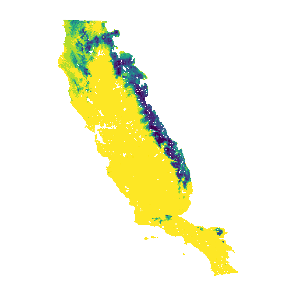
Constrain the model with msdm_posterior
Finally, flexsdm offers users function that help correct overprediction of SDM based on occurrence records and suitability patterns. In this example we constrained the ensemble model using the method “occurrence based restriction”, which assumes that suitable patches that intercept species occurrences are more likely a part of species distributions than suitable patches that do not intercept any occurrences. Because all methods of the msdm_posteriori() function work with presences it is important to always use the original database (i.e., presences that have not been spatially or environmentally filtered). All of the methods available in the msdm_posteriori() function are based on Mendes et al. (2020).
thr_val <- ens_m$performance %>%
dplyr::filter(threshold == "max_sens_spec") %>%
pull(thr_value)
m_pres <- msdm_posteriori(
records = abies_p,
x = "x",
y = "y",
pr_ab = "pr_ab",
cont_suit = pr_1$meanw[[1]],
method = c("obr"),
thr = thr_val,
buffer = NULL
)
cl <- c("#FDE725", "#B3DC2B", "#6DCC57", "#36B677", "#1F9D87", "#25818E", "#30678D", "#3D4988", "#462777", "#440154")
plot(m_pres[[1]], col = cl, legend = FALSE, axes = FALSE)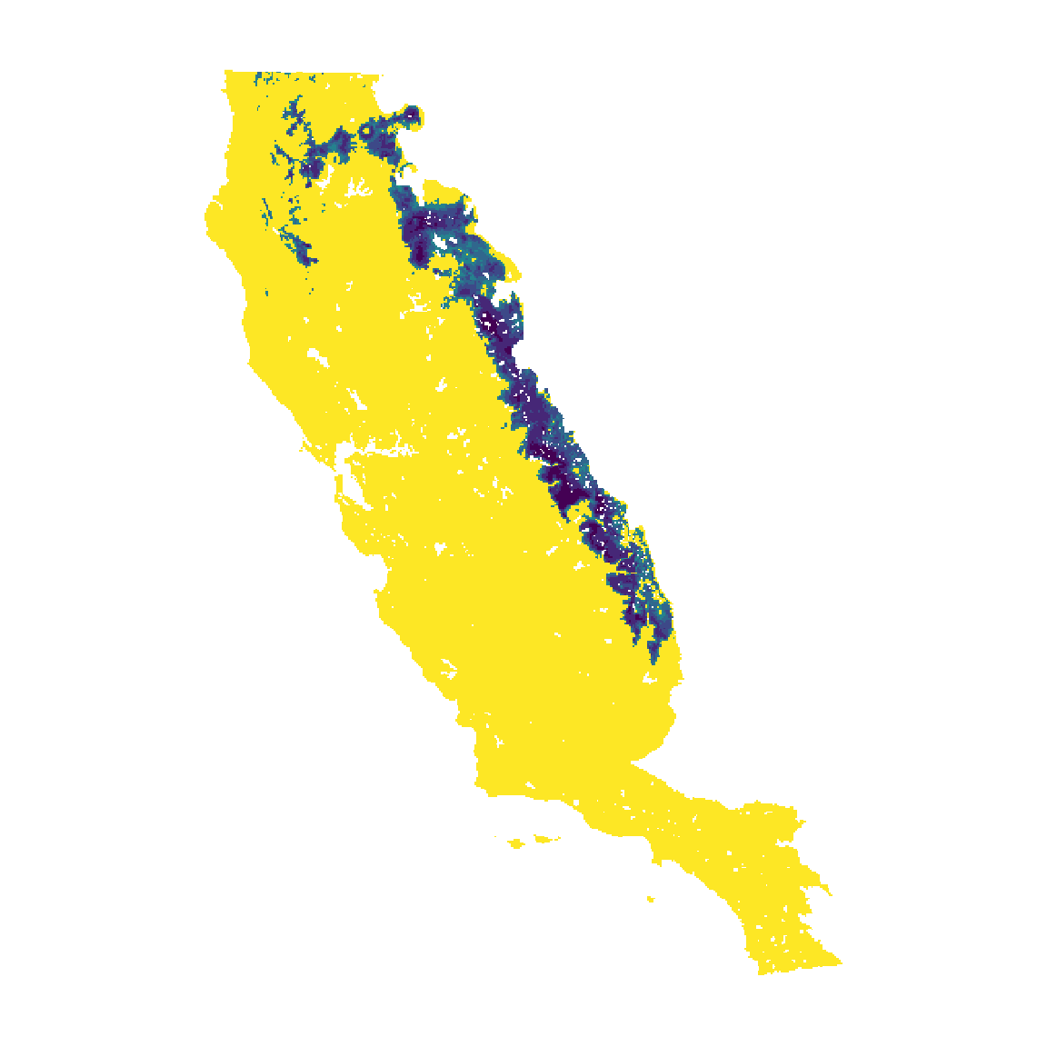 #=========#=========#=========#=========#=========#=========#=========#
Vignette still under construction and changes
#=========#=========#=========#=========#=========#=========#=========#