flexsdm: Tools to explore extrapolation in SDMs
Source:vignettes/v06_Extrapolation_example.Rmd
v06_Extrapolation_example.RmdIntroduction
Many SDM applications require model extrapolation, e.g., predictions beyond the range of the data set used to fit the model. For example, models often must extrapolate when predicting habitat suitability under novel environmental conditions induced by climate change or predicting the spread of an invasive species outside of its native range based on the species-environment relationship observed in its native range.
In flexsdm, we offer a new approach (known as Shape) for evaluating the extrapolation and truncating spatial predictions based on the degree of extrapolation measured. Shape is a model-agnostic approach for calculating the degree of extrapolation for a given projection data point by its multivariate distance to the nearest training data point – capturing the often complex shape of data within environmental space. These distances are then relativized by a factor that reflects the dispersion of the training data in environmental space. As implemented in flexsdm, the Shape approach also incorporates an adjustable threshold to allow for binary discrimination between acceptable and unacceptable degrees of extrapolation, based on the user’s needs and applications. For more information about Shape metric, we recommend reading the article Velazco et al., 2023.
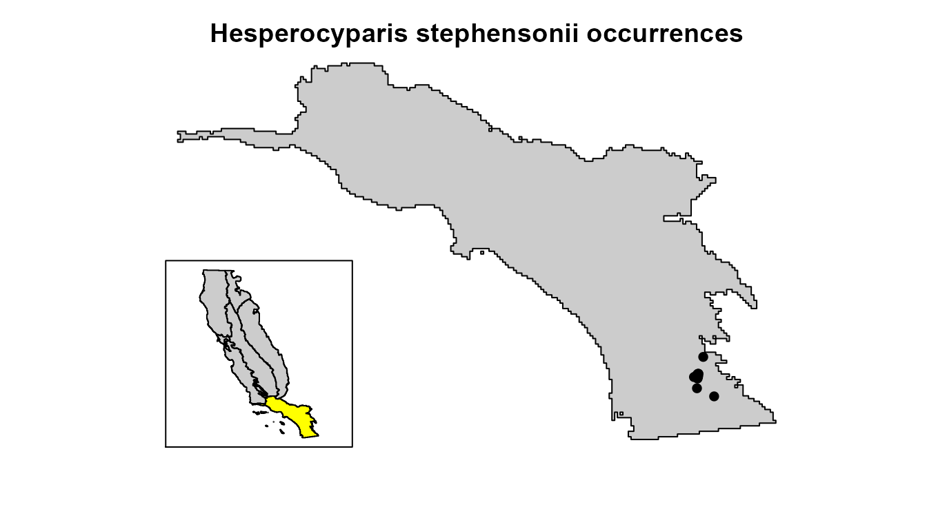
In this vignette, we will walk through how to evaluate model extrapolation for Hesperocyparis stephensonii (Cuyamaca cypress), a conifer tree species that is endemic to southern California. This species is listed as Critically Endangered by the IUCN and has an extremely restricted distribution, as it is only found in the headwaters of King Creek in San Diego County.
Note: this tutorial follows generally the same workflow as the vignette for modeling the distribution of a rare species using an ensemble of small models (ESM). However, instead of constructing ESMs, we will evaluate model extrapolation if we were to predict our models to the extent of the California Floristic Province (CFP).
Data
For our models, we will use four environmental variables that influence plant distributions in California: available evapotranspiration (aet), climatic water deficit (cwd), maximum temperature of the warmest month (tmx), and minimum temperature of the coldest month (tmn). Our occurrence data include 21 geo-referenced observations downloaded from the online database Calflora.
library(flexsdm)
library(terra)
library(dplyr)
library(patchwork)

# environmental data
somevar <- system.file("external/somevar.tif", package = "flexsdm")
somevar <- terra::rast(somevar)
names(somevar) <- c("cwd", "tmn", "aet", "ppt_jja")

# species occurence data (presence-only)
data(hespero)
hespero <- hespero %>% dplyr::select(-id)

# California ecoregions
regions <- system.file("external/regions.tif", package = "flexsdm")
regions <- terra::rast(regions)
regions <- terra::as.polygons(regions)
sp_region <- terra::subset(regions, regions$category == "SCR") # ecoregion where *Hesperocyparis stephensonii* is found

# visualize the species occurrences
plot(
  sp_region,
  col = "gray80",
  legend = FALSE,
  axes = FALSE,
  main = "Hesperocyparis stephensonii occurrences"
)
points(hespero[, c("x", "y")], col = "black", pch = 16)
cols <- rep("gray80", 8)
cols[regions$category == "SCR"] <- "yellow"
terra::inset(
  regions,
  loc = "bottomleft",
  scale = .3,
  col = cols
)
Delimit calibration area
First, we must define our model’s calibration area. The flexsdm package offers several methods for defining the model calibration area. Here, we will use 25-km buffer areas around the presence points to select our pseudo-absence locations.
ca <- calib_area(
  data = hespero,
  x = "x",
  y = "y",
  method = c("buffer", width = 25000),
  crs = crs(somevar)
)

# visualize the species occurrences & calibration area
plot(
  sp_region,
  col = "gray80",
  legend = FALSE,
  axes = FALSE,
  main = "Calibration area and occurrences"
)
plot(ca, add = TRUE)
points(hespero[, c("x", "y")], col = "black", pch = 16)
Create pseudo-absence data
As is often the case with rare species, we only have species presence data. However, most SDM methods require either pseudo-absence or background point data. Here, we use our calibration area to produce pseudo-absence data that can be used in our SDMs.
# Sample the same number of species presences
set.seed(10)
psa <- sample_pseudoabs(
  data = hespero,
  x = "x",
  y = "y",
  n = sum(hespero$pr_ab), # number of pseudo-absence points equal to number of presences
  method = "random",
  rlayer = somevar,
  calibarea = ca
)

# Visualize species presences and pseudo-absences
plot(
  sp_region,
  col = "gray80",
  legend = FALSE,
  axes = FALSE,
  xlim = c(289347, 353284),
  ylim = c(-598052, -520709),
  main = "Presence = yellow, Pseudo-absence = black"
)
plot(ca, add = TRUE)
points(psa[, c("x", "y")], cex = 0.8, pch = 16, col = "black") # Pseudo-absences
points(hespero[, c("x", "y")], col = "yellow", pch = 16, cex = 1.5) # Presences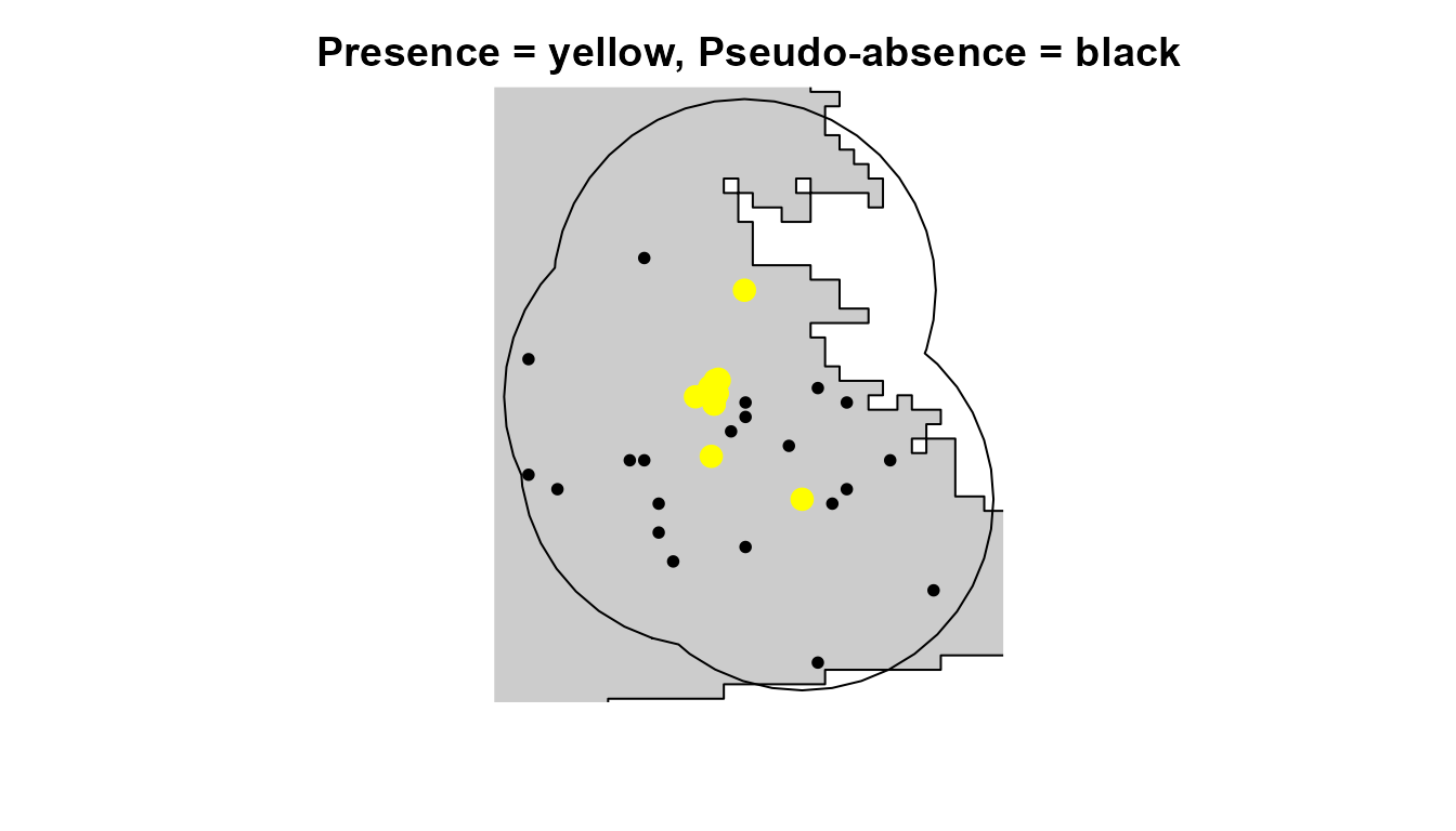
# Bind a presences and pseudo-absences
hespero_pa <- bind_rows(hespero, psa)
hespero_pa # Presence-Pseudo-absence database
#> # A tibble: 42 × 3
#>          x        y pr_ab
#>      <dbl>    <dbl> <dbl>
#>  1 316923. -557843.     1
#>  2 317155. -559234.     1
#>  3 316960. -558186.     1
#>  4 314347. -559648.     1
#>  5 317348. -557349.     1
#>  6 316753. -559679.     1
#>  7 316777. -558644.     1
#>  8 317050. -559043.     1
#>  9 316655. -559928.     1
#> 10 316418. -567439.     1
#> # ℹ 32 more rows
Partition data for evaluating models
To evaluate model performance, we need to specify data for testing and training. flexsdm offers a range of random and spatial and random data partition methods for evaluating SDMs. Here we will use repeated K-fold cross-validation, which is a suitable partition approach for validating SDM with few data.
set.seed(10)

# Repeated K-fold method
hespero_pa2 <- part_random(
  data = hespero_pa,
  pr_ab = "pr_ab",
  method = c(method = "rep_kfold", folds = 5, replicates = 10)
)
Extracting environmental values
Next, we extract the values of our four environmental predictors at the presence and pseudo-absence locations.
hespero_pa3 <-
  sdm_extract(
    data = hespero_pa2,
    x = "x",
    y = "y",
    env_layer = somevar,
    variables = c("cwd", "tmn", "aet", "ppt_jja")
  )
Modeling
Let’s use three standard algorithms to model the distribution of Hesperocyparis stephensonii: GLM, GBM, and SVM. In this case, we will use the extent of the CFP as our prediction area so that we can evaluate model extrapolation across a broad geographic area.
mglm <-
  fit_glm(
    data = hespero_pa3,
    response = "pr_ab",
    predictors = c("cwd", "tmn", "aet", "ppt_jja"),
    partition = ".part",
    thr = "max_sens_spec"
  )

mgbm <- fit_gbm(
  data = hespero_pa3,
  response = "pr_ab",
  predictors = c("cwd", "tmn", "aet", "ppt_jja"),
  partition = ".part",
  thr = "max_sens_spec"
)

msvm <- fit_svm(
  data = hespero_pa3,
  response = "pr_ab",
  predictors = c("cwd", "tmn", "aet", "ppt_jja"),
  partition = ".part",
  thr = "max_sens_spec"
)


mpred <- sdm_predict(
  models = list(mglm, mgbm, msvm),
  pred = somevar,
  con_thr = TRUE,
  predict_area = NULL
)
Comparing our models
First, let’s take a look at the spatial predictions for our models. GLM and GBM predict a lot of suitable habitat very far from where the species is found!
par(mfrow = c(1, 3))
plot(mpred$glm, main = "GLM")
# points(hespero$x, hespero$y, pch = 19)
plot(mpred$gbm, main = "GBM")
# points(hespero$x, hespero$y, pch = 19)
plot(mpred$svm, main = "SVM")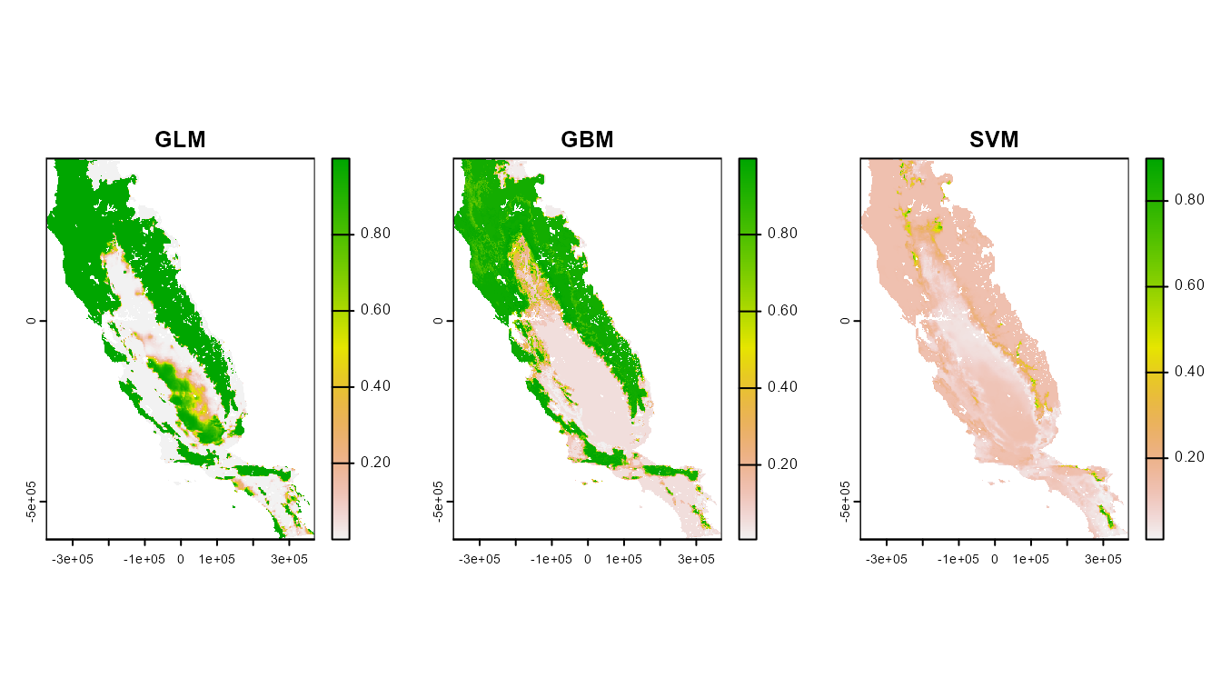
# points(hespero$x, hespero$y, pch = 19)Partial dependence plots to explore the impact of predictor conditions on suitability
Extrapolation reflects an issue with how a model handles novel data.
Here, we see that the three algorithms explored in this tutorial predict
pretty different geographic patterns of habitat suitability based on the
same occurrence/pseudo-absence data and environmental predictors. Let’s
take a look at some partial dependence plots to see that the marginal
effect of each of the environmental predictors on suitability looks like
for each of our test models. This function allows you to visualize the
how a model may extrapolate outside the environmental conditions used in
training, by visualizing the “projection” data in a different color. In
this case, that will be our environmental predictors that cover the
extent of the CFP. flexsdm allows users to plot univariate
partial dependence plots (p_pdp)
and bivariate partial dependence plots (p_bpdp);
both are shown below for each model. Note: the p_bpdp function allows
users the option to show the boundaries for the training data using
either a rectangle or convex hull approach. Here we will use the convex
hull approach.
Uni and bivariate partial dependence plots for the GLM:
p_pdp(model = mglm$model, training_data = hespero_pa3, projection_data = somevar)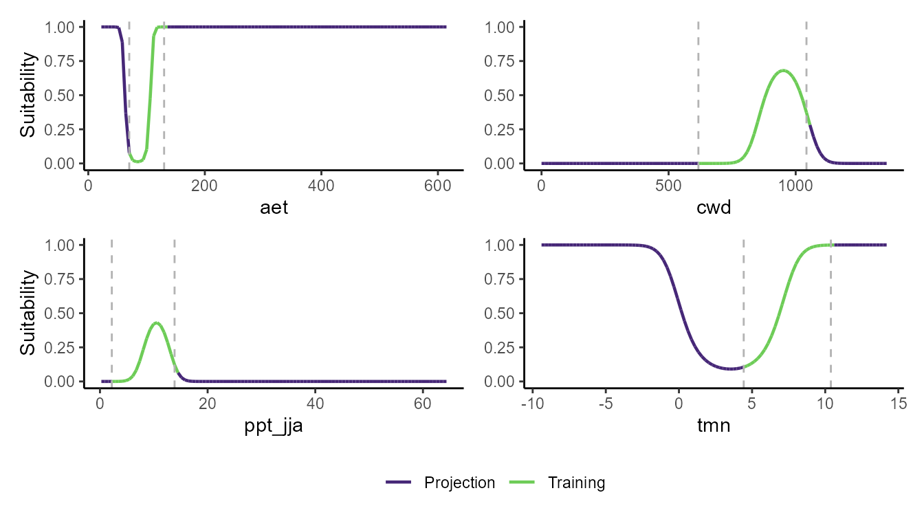
p_bpdp(model = mglm$model, training_data = hespero_pa3, training_boundaries = "convexh")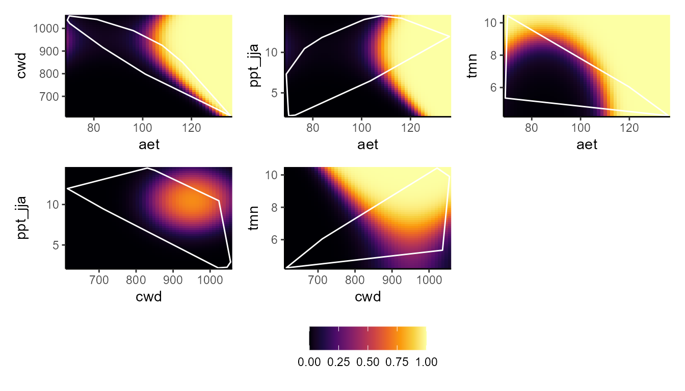
Uni and bivariate partial dependence plots for the GBM:
p_pdp(model = mgbm$model, training_data = hespero_pa3, projection_data = somevar)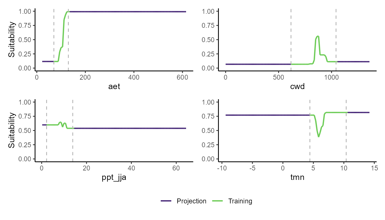
p_bpdp(model = mgbm$model, training_data = hespero_pa3, training_boundaries = "convexh", resolution = 100)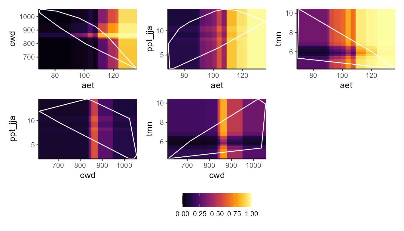
Uni and bivariate partial dependence plots for the SVM:
p_pdp(model = msvm$model, training_data = hespero_pa3, projection_data = somevar)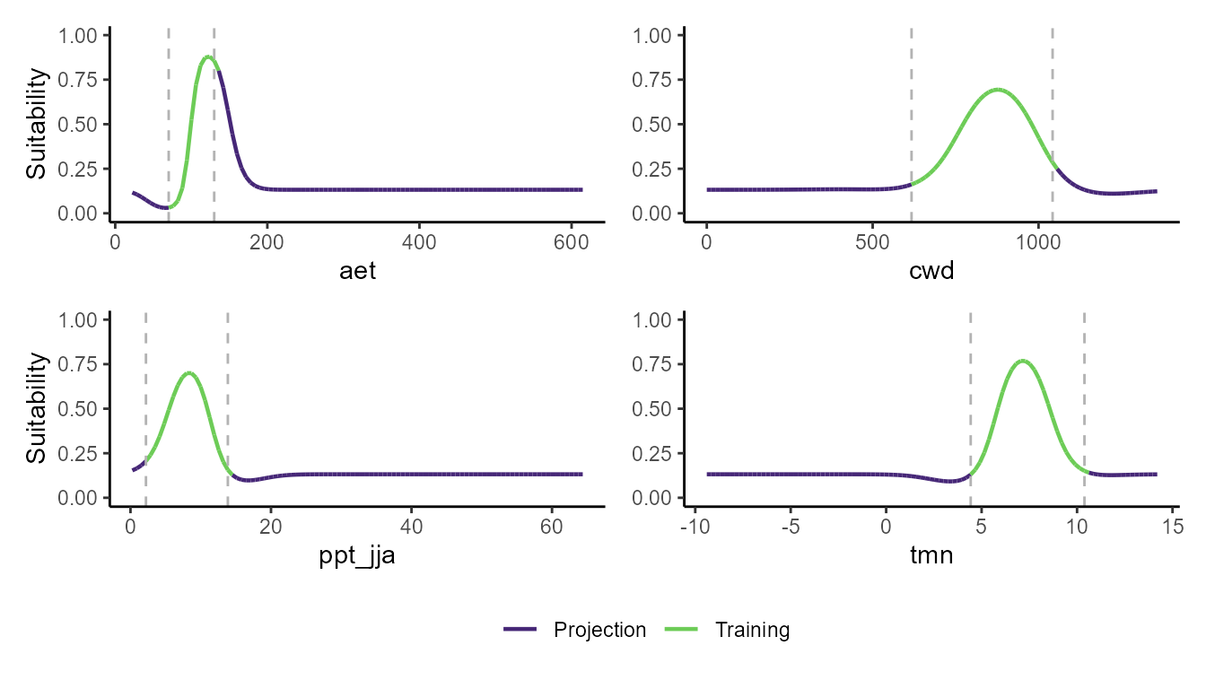
p_bpdp(model = msvm$model, training_data = hespero_pa3, training_boundaries = "convexh")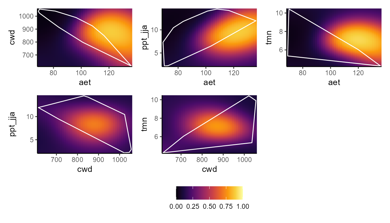
These plots show a really interesting story! Most notably, the GLM and GBM show consistently high habitat suitability for those areas that have much higher actual evapotranspiration than the very narrow range of values that were used to train the model. However, the SVM seems to do the best job of not estimating very high habitat suitability for environmental values that were outside of the training data. Importantly, these models can behave very differently depending on the modeling situation and context.
Extrapolation evaluation
Remember that our species is highly restricted to southern California! However, two of our models (GLM and GBM) predict very high habitat suitability throughout other parts of the CFP, while the SVM provides more conservative predictions. We see that GLM and GBM tend to predict high habitat suitability in those areas that are very environmentally different from our training conditions. But where are our models extrapolating in environmental space? Let’s find out using the “extra_eval” function in SDM. This function requires you to input the model training data, a column specifying presence vs. absence locations, projection data (can be a SpatRaster or a tibble containing data used for model projection – this can reflect a larger region, separate region, or different time period than what was used for model training), a metric for calculating the degree of extrapolation (the default is Mahalanobis distance, though euclidean is also an option- we will explore both), number of cores for parallel processing, and an aggregation factor, in case you want to measure extrapolation for a very large data set.
First we look at the degree of extrapolation in geographic space using the Shape method based on Mahalanobis distance. Also we will distinguish between univariate and combinatorial extrapolation.
Using Mahalanobis distance:
xp_m <-
  extra_eval(
    training_data = hespero_pa3,
    pr_ab = "pr_ab",
    projection_data = somevar,
    metric = "mahalanobis",
    univar_comb = TRUE,
    aggreg_factor = 1
  )
xp_m
#> class       : SpatRaster
#> size        : 558, 394, 2  (nrow, ncol, nlyr)
#> resolution  : 1890, 1890  (x, y)
#> extent      : -373685.8, 370974.2, -604813.3, 449806.7  (xmin, xmax, ymin, ymax)
#> coord. ref. : +proj=aea +lat_0=0 +lon_0=-120 +lat_1=34 +lat_2=40.5 +x_0=0 +y_0=-4000000 +datum=NAD83 +units=m +no_defs
#> source(s)   : memory
#> varnames    : somevar
#>
#> names       : extrapolation, uni_comb
#> min values  :             0,        1
#> max values  :    3730.67743,        2
The output of the extra_eval function is a SpatRaster, showing the degree of extrapolation across the projection area, as estimated by the Shape method.
cl <- c("#FDE725", "#B3DC2B", "#6DCC57", "#36B677", "#1F9D87", "#25818E", "#30678D", "#3D4988", "#462777", "#440154")

par(mfrow = c(1, 2))
plot(xp_m$extrapolation, main = "Shape metric", col = cl)
plot(xp_m$uni_comb, main = "Univariate (1) and \n combinatorial (2) extrapolation", col = cl)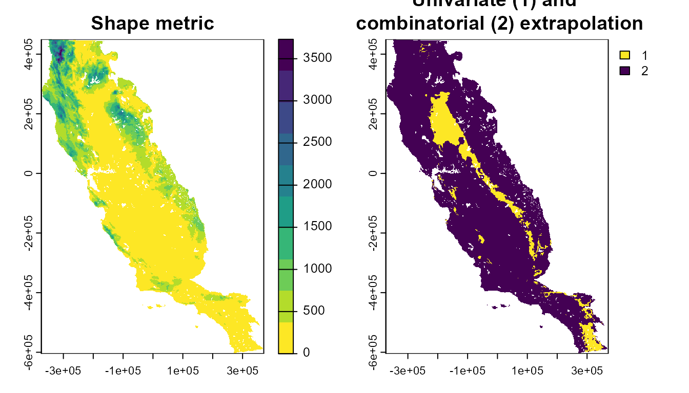
We can also explore extrapolation or suitability patterns in
environmental and geographic space, using just one function. To do that,
we will use the p_extra
function. This function plots a ggplot object.
Let’s start with our extrapolation evaluation. These plots show that areas with high extrapolation (dark blue) are far from the training data (shown in black) in both environmental and geographic space.
The higher extrapolation values extrapolation area in the northwestern portion of the CFP.
p_extra(
  training_data = hespero_pa3,
  x = "x",
  y = "y",
  pr_ab = "pr_ab",
  color_p = "black",
  extra_suit_data = xp_m,
  projection_data = somevar,
  geo_space = TRUE,
  prop_points = 0.05
)
#> Number of cell used to plot 3642 (5%)
Let’s explore univariate and combinatorial extrapolation. The former is defined as the projecting data outside range of training conditions, while the combinatorial extrapolation area those projecting data within the range of training conditions.
p_extra(
  training_data = hespero_pa3,
  x = "x",
  y = "y",
  pr_ab = "pr_ab",
  color_p = "black",
  extra_suit_data = xp_m$uni_comb,
  projection_data = somevar,
  geo_space = TRUE,
  prop_points = 0.05,
  color_gradient = c("#B3DC2B", "#30678D"),
  alpha_p = 0.2
)
#> Number of cell used to plot 3642 (5%)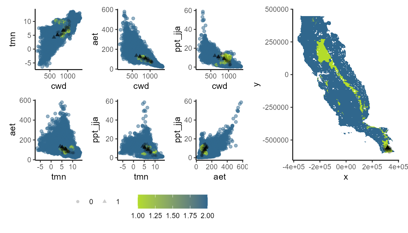
Truncating SDMs predictions based on extrapolation thresholds
Depending on the user’s end goal, you may want to exclude suitability values that are environmentally “too” far from modeling training data. The Shape method allows you to select any extrapolation threshold to exclude suitability values.
Before truncating our models we can use the p_extra
function to explore binary extrapolation patter in the environmental and
geographical space. Here we will test the values 50, 100, and 500, for
comparison.
p_extra(
  training_data = hespero_pa3,
  x = "x",
  y = "y",
  pr_ab = "pr_ab",
  color_p = "black",
  extra_suit_data = as.numeric(xp_m$extrapolation < 50),
  projection_data = somevar,
  geo_space = TRUE,
  prop_points = 0.05,
  color_gradient = c("gray", "#FDE725"),
  alpha_p = 0.5
) + plot_annotation(subtitle = "Binary extrapolation pattern with using a threshold of 50")
#> Number of cell used to plot 3642 (5%)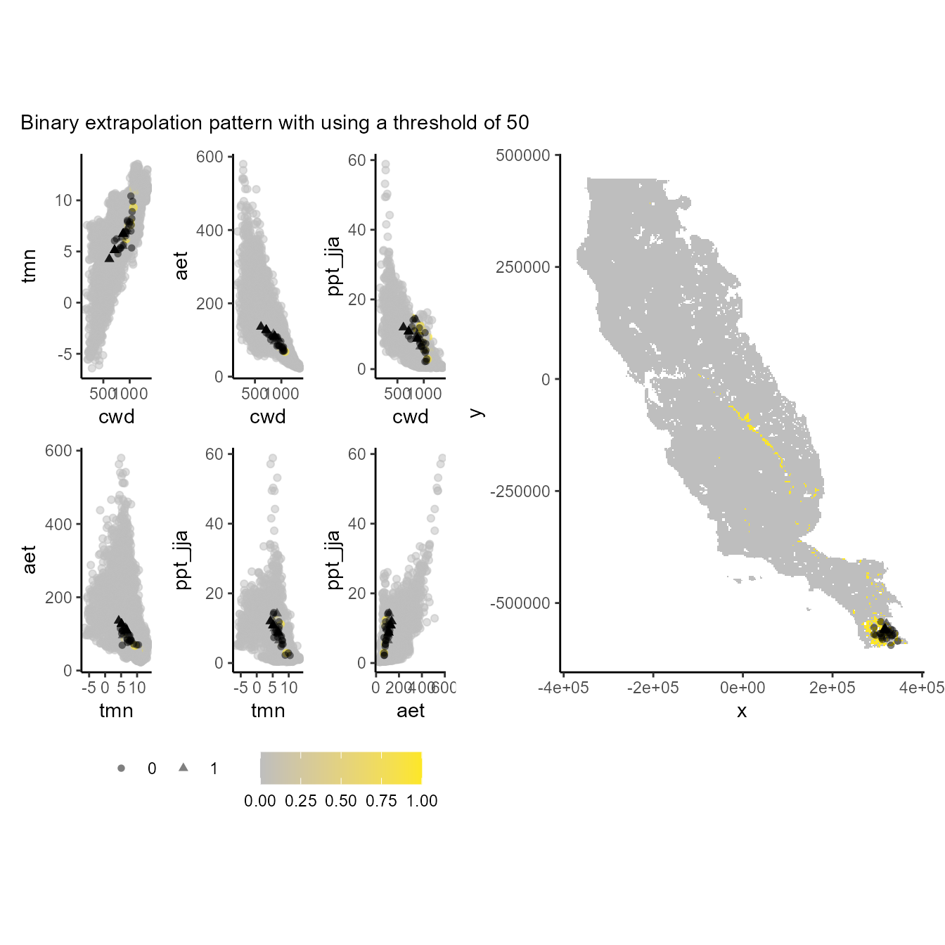
p_extra(
  training_data = hespero_pa3,
  x = "x",
  y = "y",
  pr_ab = "pr_ab",
  color_p = "black",
  extra_suit_data = as.numeric(xp_m$extrapolation < 100),
  projection_data = somevar,
  geo_space = TRUE,
  prop_points = 0.05,
  color_gradient = c("gray", "#FDE725"),
  alpha_p = 0.5
) + plot_annotation(subtitle = "Binary extrapolation pattern with using a threshold of 100")
#> Number of cell used to plot 3642 (5%)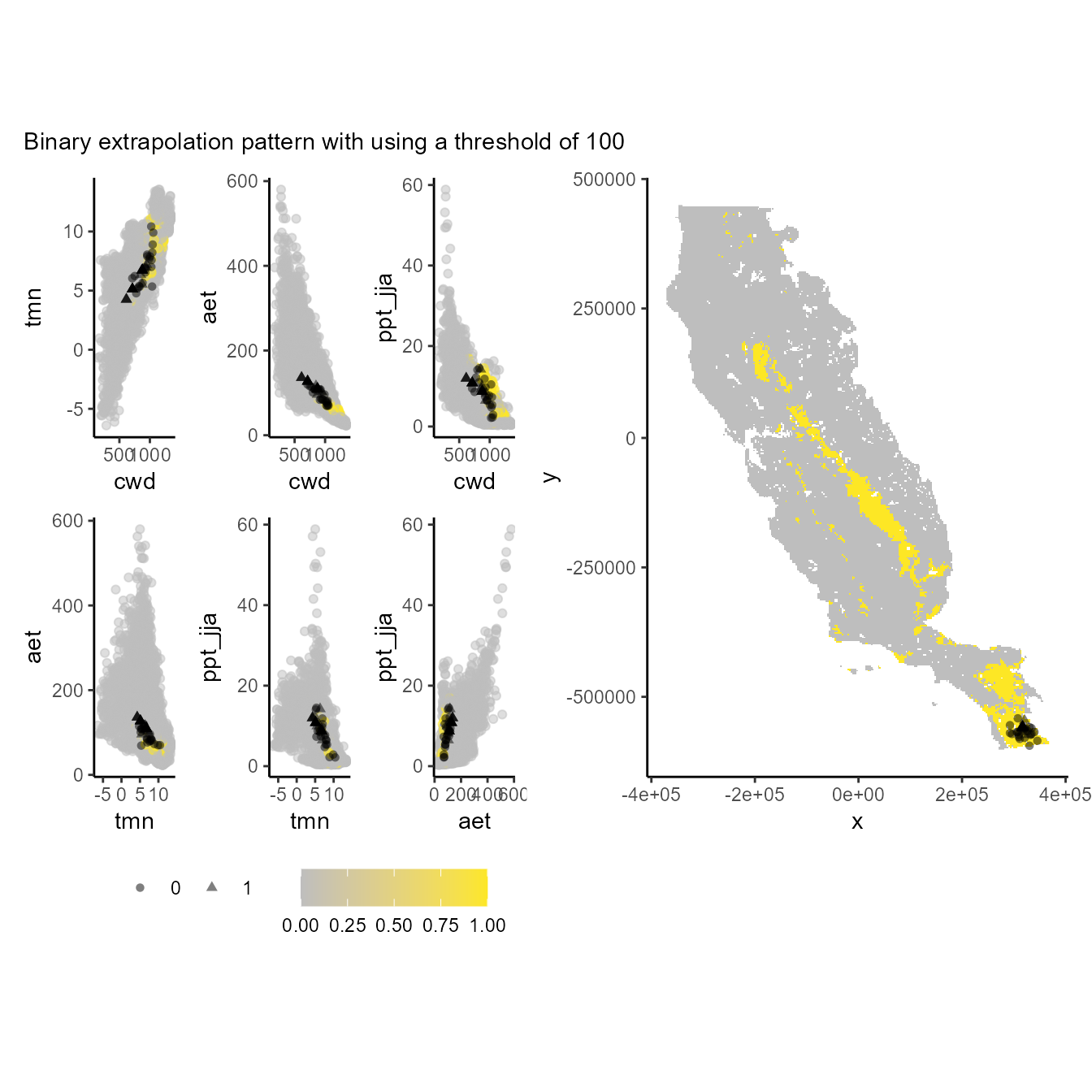
p_extra(
  training_data = hespero_pa3,
  x = "x",
  y = "y",
  pr_ab = "pr_ab",
  color_p = "black",
  extra_suit_data = as.numeric(xp_m$extrapolation < 500),
  projection_data = somevar,
  geo_space = TRUE,
  prop_points = 0.05,
  color_gradient = c("gray", "#FDE725"),
  alpha_p = 0.5
) + plot_annotation(subtitle = "Binary extrapolation pattern with using a threshold of 500")
#> Number of cell used to plot 3642 (5%)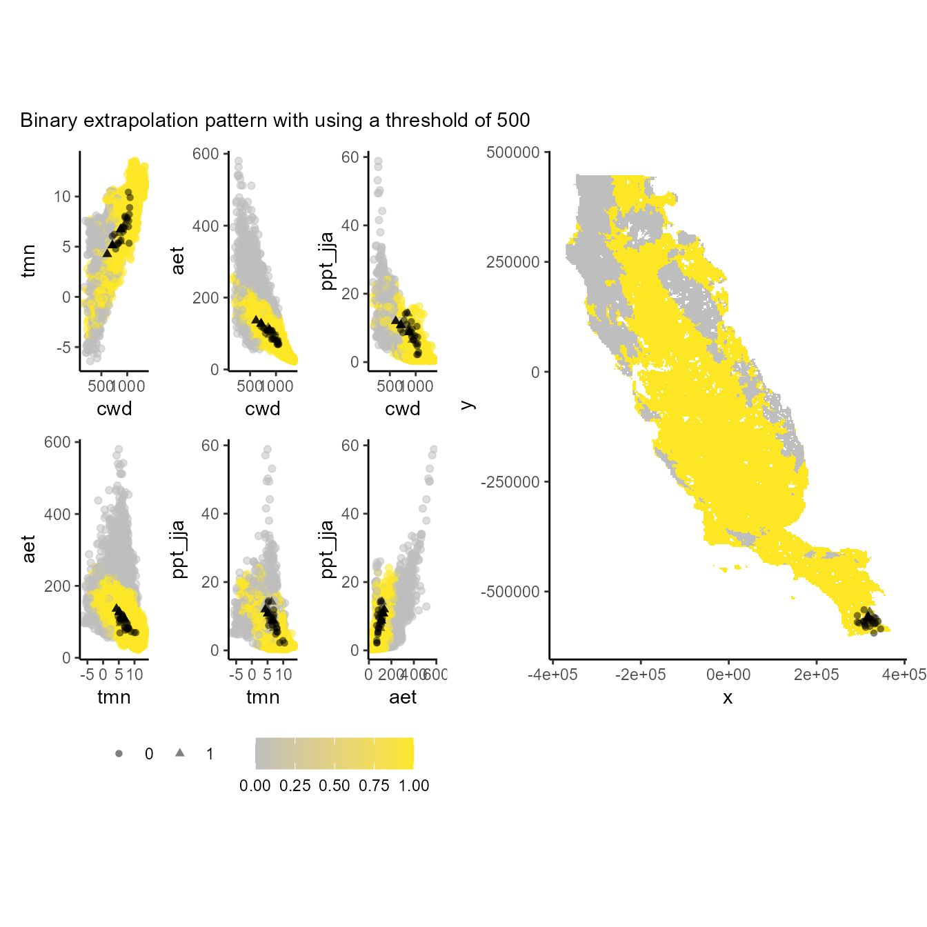
Values of 1 (yellow one) depict the environmental and geographical regions will constraint our models suitability (truncate). Note that the lower the threshold, the more restrictive the environmental and geographic regions used to constrain the model.
Now we will use the function extra_truncate
to truncate the suitability predictions made by GLM, GBM, and SVM based
on extrapolation thresholds explored previously. As a note, threshold
selection will be very user-dependent, but this function allows you to
select multiple thresholds at one time to compare outputs. Users can
also select a “trunc_value” within the extra_truncate function, that
specifies the value that should be assigned to those cells that exceed
the extrapolation threshold (also specified in the function). The
default is 0 but users could also choose another value for which to
reduce suitability.
glm_trunc <- extra_truncate(
  suit = mpred$glm,
  extra = xp_m,
  threshold = c(50, 100, 500),
  trunc_value = 0
)

gbm_trunc <- extra_truncate(
  suit = mpred$gbm,
  extra = xp_m,
  threshold = c(50, 100, 500),
  trunc_value = 0
)

svm_trunc <- extra_truncate(
  suit = mpred$svm,
  extra = xp_m,
  threshold = c(50, 100, 500),
  trunc_value = 0
)
par(mfrow = c(3, 3))
plot(glm_trunc$`50`, main = "GLM; extra threshold = 50", col = cl)
plot(glm_trunc$`100`, main = "GLM; extra threshold = 100", col = cl)
plot(glm_trunc$`500`, main = "GLM; extra threshold = 500", col = cl)
plot(gbm_trunc$`50`, main = "GBM; extra threshold = 50", col = cl)
plot(gbm_trunc$`100`, main = "GBM; extra threshold = 100", col = cl)
plot(gbm_trunc$`500`, main = "GBM; extra threshold = 500", col = cl)
plot(svm_trunc$`50`, main = "SVM; extra threshold = 50", col = cl)
plot(svm_trunc$`100`, main = "SVM; extra threshold = 100", col = cl)
plot(svm_trunc$`500`, main = "SVM; extra threshold = 500", col = cl)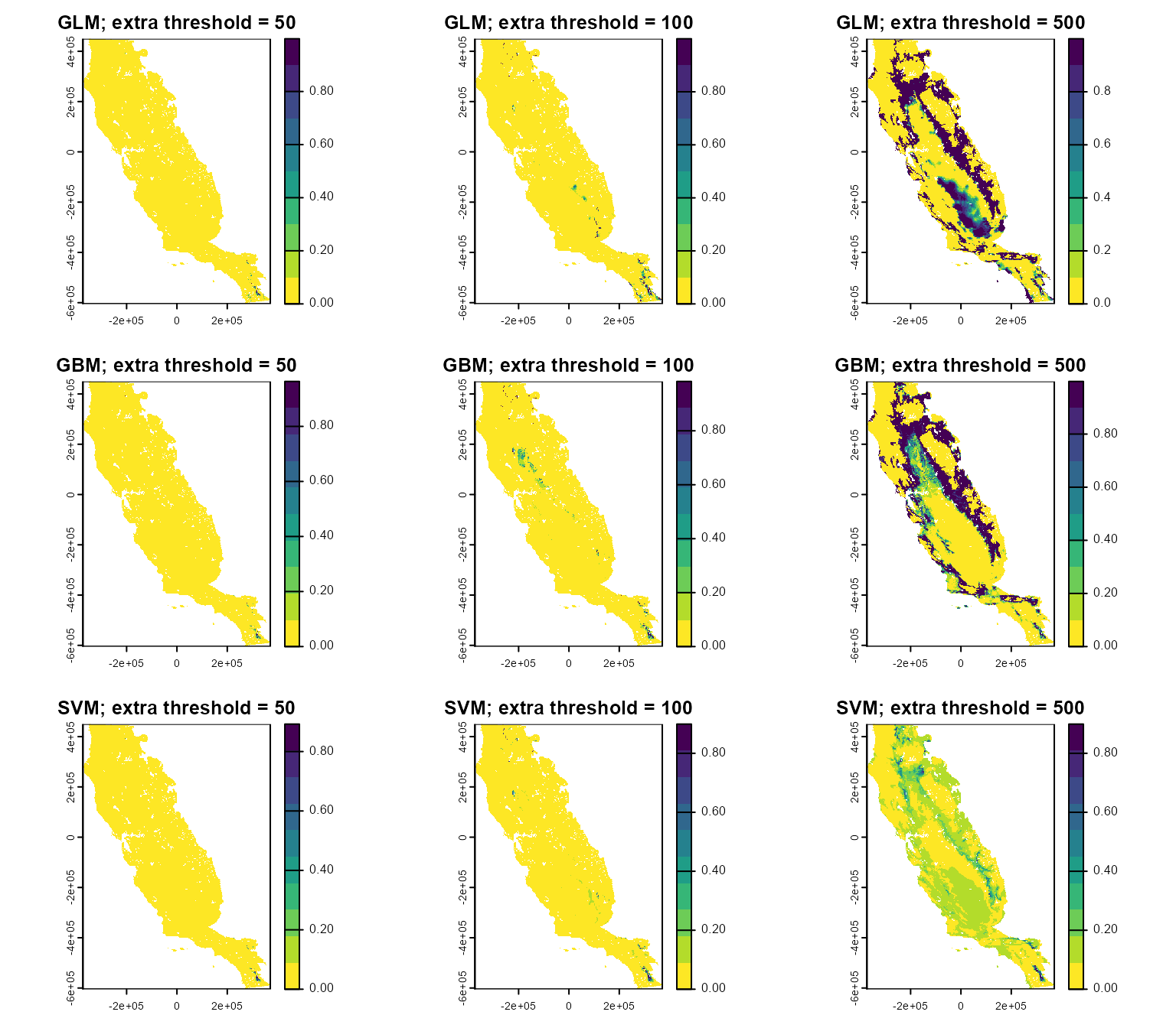
Based on these maps, you can see that the lower the extrapolation threshold, the more restricted the habitat suitability patterns, while higher values retain a greater amount of suitable habitat. Selecting the best threshold will depend on modeling goals and objectives, and .
Want to learn more about Shape and other extrapolation metrics? Read the article “Velazco, S. J. E., Brooke, M. R., De Marco Jr., P., Regan, H. M., & Franklin, J. (2023). How far can I extrapolate my species distribution model? Exploring Shape, a novel method. Ecography, 11, e06992. https://doi.org/10.1111/ecog.06992”